Transkriptio

1

2

3

4

5

6

7

8

9

10

11

12

13

14

15

16

17

18

19

20

21

22

23

24

25

26 ̹ ½º ¼ ¼Ì ØÓ ÓÒ Ò ÃÓÖÖ Ð Ø ÓÑ ØÖ ÓÚ Ö Ò Ñ ØÖ Ô ÓÑÔÓÒ ÒØØ Ò ÐÝÝ Å Ö Ù È ÙÖ ½ x 2 Ì Ø ÐÐÒÑÙÙØ Ñ Ñ Ø Ñ ØØ Ø ØÝ ÐÙ Ó ÐÐ Ò ÐÚ ÐÐ ÒÒ ØÙÒÚ ØÓÖ ÓÙ ÓÒ Ó ¹ x x 1 ÝѺ Ó ØÙ Ò ÚÝÒØÙÑÑÙÙ Ú Ø Ð Ñ ÐÐ ÒÔ ÐÐÓÐÐ ºÎÓ Ò Ù Ø Ò ÒÓÐ ØØ ØØ Ø ÚÖ ¹ Ò Ò Ò Ú Ò ÝÝ ÐÓ Ù Ò Ò ÐØ ÚÝ Ò ÒÚ Ð Ô ÐØÓ ÙÑÑ ÐÐ Ò Ò Ú ÐÐ ºÎ Ð ÒÐ ÓÓÒØÙÑ Ø ÚÝ Ð Ø ÐÐ Ø ÒÔ Ö Ô Ø Ú ØÚ Ö Ò ÔÙÒ Ò Ó ØÙ Ù ÔÝ ÝÝ ÙÙÒÒ ÐÐ ÒÚ ÓÒ º ÐÐ TºÅ Ð Ø ÐÐ ØØ Ò ÒÒ ØÙ Ñ Ö ÓÒ Ñ Ö Ú Ö ÔÙÒ ¹ TÚÓ ÓÐÐ Ø ÒÓÑ Ò ÙÙ ºÃÙÚ Ò ØØ ÐÝÒØ Ô Ù ØÙØ ØØ Ú Ú ØÓÖ Ü=[x 1 x 2 x n ] Ñ Ö Ø ÐÐ ØØ ÙÚ Òf Ö Ù Ö Ò Ú ÐÐ 1,2,...,nÔ Ø (i,j)ºìðð Ò Ü=Ü(i,j) = [f 1 (i,j) f 2 (i,j) 2µº f n (i,j)] 1µ ÔÙÒ ÐÐ ½ ÃÓÖÖ Ð Ø Ó ÓÐ Ú ÙÚ ÚÓ ÓÐÐ Ø Ò Ñ Ö ÙÖ Ô ÐÐÓÒ ÚÝ Ò ÝØØÝØÝÑ ØÚ Ö ÐÐ x Ò Ú ÐÐ x ÃÓÖÖ Ð Ø ÓÑ ØÖ Ã ÙÚ Ú ØÓÖ ÑÙÙØØÙ Ò ÓÑÔÓÒ ÒØØ Ò ÝØØÝØÝÑ Ø º ººº º E{x 1 x 1 } E{x 1 x 2 } E{x 1 x n } ÃÜ= E{ÜÜT E{x 2 x 1 } E{x 2 x 2 } E{x 2 x n } } = Ô ÐØÓ ØØÚ Ô Ð ØÔÙÒ Ò Ò Ú Ö Ú Ø Ð Ú Ø Ò Ú ÐÐ Ò Ù Ø Ò Ò ÙÒ ÃÓÖÖ Ð Ø ÓÑ ØÖ Ð Ø Ò ÓÑÔÓÒ ÒØØ Ò Ò Ø ÒØÙÐÓ ÒÓ ÓØÙ ÖÚÓ ºÂÓ ØÙØ ØØ ¹ E{x n x 1 } E{x n x 2 } E{x n x n } Ø Ò Ò Ò ÚÝ Ñ Ö Ú Ö ÒÖ ÖÙÓ Ó Ò Ò Ò ÒÚÖ ÓÑÔÓÒ ÒØØ Ú ÖÑ Ò Ò Ö 2µÚ Ø Ð Ú Ø Ñ ÒØ Ø Ò Ò ØÚ Ø Ú Ø Ø Ò Ö Ø Ó ÒØÙÒ ÑÙÙØ Ò ÐÐ Ò ÚÝ Ô ÐÐÓ º }ÓÒÒÓÐÐ Ø ÔÓ Ú º Ñ Ö ÐØ Ø ÙÖ ¹ Ú ÐÑ ÓÑÔÓÒ ÒØØ ÑÙÙØØ٠Ѻx 1 x ÓÖÖ Ð Ø ÓÑ ØÖ Ò ÓÑÔÓÒ ÒØØ k 12 = E{x 1,x Ù ÑÑ Ø ÒÔÓ Ø Ú Ò Ø Ú Ø ÓÖÖ Ð Ø ÓØ ÝÒÒݺµ Ñ Ö Ò Ø Ú Ø Ö Ð Ñ Ð¹ ÔÙÓÐ Ø Ð ÓØÓÚ ØÝÐ Ø Ô Ù ÑÝ Ò Ø Ú º ÃÙÚ Ò ØØ ÐÝ Ô Ð Ò ÖÚÓØÓÚ Ø ÃÓÖÖ Ð Ø ÓÑ ØÖ Ò ÓÒ Ð ÓÒ Ö Ð ÑÙÙØØÙ ÐÐ µ Ò ¹Ò Ø Ú Ò Ò ÑÙØØ ÓÒ Ð ÒÙÐ Ó¹ 2 ¾ = Ô Ð ÒØÙÑ Ò Ó Ø Ú Ñ Ø Ñ Ò ÓÖÖ Ð Ø Ó Ø ÚÓ ÓÐÐ x 1 = ÖÙÙ Ò ÐÝØÝ ÐÑÔ Ø Ð x 2

27 ÝØØ Ô Ú Ø Ø ÒÔ ÒÐ ØØÙÒ ºÃÓÖÖ Ð Ø ÓÑ ØÖ ÓÒÑ Ð ÓÚ ØÙÐ Ø ÐÑÑÖ Ø º ÇÐ Ø Ø Ò ØØ Ð ÙÔ Ö ÐÐ Ø ÐÐ ÜØ ÒÐ Ò Ö Ò ÒÑÙÙÒÒÓ ÖØÓÑ ÐÐ Ñ ØÖ ÐÐ Ý= ܺ ÃÝØÒÒ Ú Ò Ñ Ò ÓÖÖ Ð Ø ÓÑ ØÖ Ò Ð Ó Ø ÓÒÑ Ð ØÚ ÖØ ÐÐ ÒÒºÂÓ Ø Ô Ù ¹ ij ÖØÓÓ ØØÑÙÙØØÙ ÐÐ i jóò ÓØ ÒÔ Ð ÒÒº T ÐØ Ò Ò Ò Ú Ö Ú Ð Ó Ò Òµ Ø ÑÑ ÒÚ Ô ÙÖ Ú Ø T ÔÙÒ Ò Ò Ú Ö ÙÙÖ Ø ÖÚÓ Ð ÓÐÐ k ÂÓ Ñ Ö ÐÙ ÑÑ ÑÙÙØØ Ø ÐÐ Ø Ò Ð ÙÔ Ö Ø Ò Ú ØÜ=[x 1 x 2 x 3 ] Ò Ò Òµ Ò Ú Ý=[y 1 y 2 y 3 ] Å ØÖ ÐÐ ÖØÓÑ ÐÐ ÙÒÙÙ ÒÑÙÙØØÙ ÒÝ ÓÖÖ Ð Ø ÓÑ ØÖ ÓÒ 1/ 2 1/ 2 0 Ý= = 0 1/ 2 1/ x 1 2 1/ 3 1/ 3 1/ x 2 3 x ÌÑØ Ö Ó ØØ Ø ØØ ÓÑÔÓÒ ÒØ Ø ØÙÐ ÓÖÖ ÐÓ Ñ ØØÓÑ Ð Ò ÚØ ÐÐÐ Ò Ö ÂÓ Ù ØØ ÓÐÐ ØÓ ÚÓØØÙ ØØ ÐÙØÙÒÙÙ ÒÑÙÙØØÙ Ò ÓÖÖ Ð Ø ÓÑ ØÖ ÃyÓÒ ÓÒ Ð Ò Òº 3 ÚÜi Ð ÔÙ Ø Ñ ØÖ ÑÙÓ Ó 1,...,n Ó ÐÐ ÔØ ÃÝ= E{ÝÝT } = E{( Ü)( ÜT )} = E{ ÜÜT T } = E{ÜÜT } T = ÃÜ T. Ö ÔÔÙÚÙÙ ºÌ ÑÔÔÙÓÒÒ ØÙÙ ÝØØÑÐÐÃÜ ÒÓÑ Ò Ú ØÓÖ Ø ÚÜi,i = ÃÜÚÜi = λüiúüi Ù Ø Ú Ø ÙÙÒØ Ó Ãy ÔÝ ØÝ ÒØÑÒÚ ØÓÖ Ú Ò ÓÖ ÒØ Ò Ð Ñ ÒºÃÓ λü1 0 0 ÓÖÖ Ð Ø ÓÑ ØÖ ÓÒ ÝÑÑ ØÖ Ò Ò Ö Ð Ò Ò ÒÓÑ Ò Ú ØÓÖ ØÓÚ Ø Ò ÓÖØÓ ÓÒ Ð ºÂÓ ÃÜ[ÚÜ1ÚÜ2ÚÜ3] = [ÚÜ1ÚÜ2ÚÜ3] 0 λü2 0 ÚÜi ØÝÝÐ Ò λünºçñ Ò Ú ØÓÖ Ø 0 0 λü3 ÇÑ Ò ÖÚÓØλÜi ÐÑÓ Ø Ø ÒÝÐ Ò ÙÙÖ ÑÑ Ø Ô Ò ÑÔÒ λü1 λü2... ÓÒÚ Ø ØØÝÃÜ ÒÒÓÖÑ Ð Ó Ù Ø ÓÑ Ò ÖÚÓÚ ØÓÖ Ø Üi =ÚÜi Ø Ô ØÙÙ ÓÖÖ Ð Ø ÓÐÐ = TÜ1 TÜ2, TÜ3 λü1 0 0 Ñ ÓÑ Ò Ú ØÓÖ ÒÓÖØÓÒÓÖÑ Ð ÙÙ Ø ÙÖ ÃÝ= ÃÜ T = Ãx [ Ü1 Ü2 Ü3] = [ Ü1 Ü2 Ü3] 0 λü λü3 λü1 0 0 = TÜ1 TÜ2 [ Ü1 Ü2 Ü3] 0 λü2 0, TÜ3 0 0 λü3 ¾ λü1 0 0 λü1 0 0 ÃÝ= λü2 0 = 0 λü λü3 0 0 λü3

28 ÃÓÖÖ Ð Ø ÓÑ ØÖ Ò ÓÒ Ð Ó ÒØ ØÙÓØØ ÙÙ Ò ÓÓÖ Ò Ø ØÓÒ ÓÒ Ô Ð 1Ó Ó ØØ ÙÙÒØ Ô Ð ÓÒ Ó ÐØ Ò Ò ÚÝÓÒÓÖ Ò ÒØ ÐÐ ÒÚ Ö ÒÔ ÒºÅÙÙÒÒÓ Ø ÒÔ ÒÓÒÓÖØÓÒÓÖÑ Ð ¹ ÒØ Ò Ø ØØ ØÓ Ò Ò Ð ÐÑÓ ØØ ÐÑ Ø ÓÒ ÒÐ Ò ÚÝÒ Ô ÐØ ÙÙ Ò Ð Ñ Ø Ò ÐÐ Ñ Ö ØØÚ ÙÙÒØ Ò º Ñ Ö ÒØ Ô Ù Ü ÒÔÖÓ Ø ÓÔ Ð ÐÐ Ü1ÓÐ ÐÚ Ø Ò ÐØ Òµ Ñ Ú ØÓÖ ØÒÝØØÚØÓÐ Ú ÒÓÖ Ó Ø Ø ÓØØÙÒ ºÇÖØÓ ÓÒ Ð ÐÐ ØÓ ÐÐ Ð ÐÐ 2 Ú ÑÑÒ = T ÓØ ÒÜ= 1Ý= Tݺ ÙÙ Ò Ò Ó Ø ÙÓÖ Ú Ú Ò Ò 1 x 2 ¾ ÃÓÚ Ö Ò ex 2 ex1 x Ò ÒÚÓ ÒÓ ÔÓÒÒ Ø Ú ÒÓÖ Ó Ø º ÌÓ Ò ÒÓÖ ÓÓÒ Ø Ò ÒÒ ÐØ Ñ Ö ØÝ Ø ÒÔ Ø ºÌÓ Ò ÒÓ Ò ÖÚÓØÜ ÐÐÙÚ Ø ÐÑ 1 x 2 2 x x ÃÓÚ Ö Ò Ñ ØÖ ÙÚ Ú ØÓÖ ÑÙÙØØÙ Ò ÓÑÔÓÒ ÒØØ Ò ÝØØÝØÝÑ ØÒ ÒÔ ÒÓÔ Ø Ø E{Ü} Ø ÓØØÙÒ m x x x 1 1 +ÑÜÑTÜ=ÃÜ ÑÜÑTÜ ÑÜÑTÜ+ÑÜÑTÜ ÑÜ= Ü= E{(Ü ÑÜ)(Ü ÑÜ) T } = E{ÜÜT } E{ÜÑTÜ} E{ÑÜÜT } + E{ÑÜÑTÜ} =ÃÜ E{Ü}ÑTÜ ÑÜE{ÜT } E{x 1 x 1 m x1 m x1 } E{x 1 x 2 m x1 m x2 } E{x 1 x n m x1 m xn } E{x =ÃÜ ÑÜÑTÜ= 2 x 1 m x2 m x1 } E{x 2 x 2 m x2 m x2 } E{x 2 x n m x2 m xn } E{x n x 1 m xn m x1 } E{x ¾ n x 2 m xn m x2 } E{x n x n m xn m xn } º ººº º

29 È ÓÑÔÓÒ ÒØØ Ò ÐÝÝ ÐÐ Ø Ö Ó Ø Ø Ò ÓÚ Ö Ò Ñ ØÖ ÒÓÑ Ò Ú ØÓÖ Ò ¹ ÖÚÓ ÒÐ ¹ È ÓÑÔÓÒ ÒØØ Ò ÐÝÝ ºÈ ÓÑÔÓÒ ÒØØ Ò ÐÝÝ ÔÖ Ò Ô ÐÓÑÔÓÒ ÒØ Ò ÐÝ È µøùòò Ø ÒÑÝ Ò Ñ ÐÐ Ö ØØ Ñ Ø ºÌÙÐÓ Ò ÒØ ØÓ Ø Ñ Ø Ò ÒÒ ØØÙ ÓÙ ÓÚ ØÓÖ Ø ÓÒ ÙÙÒØ ÙØÙÒÙØ Ú ÖÙÙ ¹ ÓÒ Ú ÖÙÙ ºÅÙÙØ ÑÙÓØÓØ ØÓ Ñ Ö ÝÖ ÙÓÖ ÑÙÓØÓ È ÐÐ ÚÓ È ØÙÓØØ Ø ÓÒÚ ØÓÖ Ô ÐÚ ÒÑÙÓ ÓÒÔ Ø ÙÐ ÙÙ Ø ØÑ ÒÒÓ ØÙÓÔ Ø ÙÐ ÙÙ Ã Ö ÙÒ Ò¹ÄÓ Ú ¹ÑÙÙÒÒÓ ÀÓØ ÐÐ Ò ¹ÑÙÙÒÒÓ º Ö Ø ØÝ ØµÓÑ Ò Ú ØÓÖ Ø ÖÓØØ ØÓ Ø Òº ÅÙÙÒÒÓ ÓÒÒÝØÑÙÓØÓ Ý= (Ü ÑÜ) Ñ ÓÒÖ ÒÒ ØØÙ Ü Ò ÓÑ Ò ÖÚÓ ÒÑÙ Ò Ú Ö ØØÑ ÐÐ Ð ÐÐ º ÆÝØÝ ÒØ Ô Ø ÒÜ ÓÓÖ Ò Ø ØÑܹ Ú ÖÙÙ ÓÑ Ò Ú ØÓÖ Ò Ü1 Ü2 = TÜ1 TÜ2 TÜ3, x 2 x 2 ex2 ÂÓ Ù Ø ÖÚ ØØ Ú Ò Ò ÓÖÑ Ø ÓÒ ØØÑ ÖØÑ Ø ÐÐ ØØ Ñ ºººµÖ ØØ ØØ ÝØ ØÒ e x 1 m ÍÐÓØØ ÙÙ ÒÔ Ò ÒØÑ ØÓÒ ØÙ Ñ Ö ÙÚ ÒÔ Ù ºÃÙÒÚ ØÓÖ ØÑÙÙÒÒ Ø Ò Ô Ù ÝØ ØØ Ò ÒÓ Ø Ò(Ü ÑÜ) Ò Ü1 Ò ÙÙÒØ Ø ÓÑÔÓÒ ÒØØ º Ú ÒÑÙÙØ Ñ ÙÙÖ ÒØ ÓÑ Ò ÖÚÓ Ú Ø Ú ÓÑ Ò Ú ØÓÖ Ø º Ñ Ö ÝÐÐÓÐ Ú Ò ÙÚ ÒØ ¹ x x x 1 1 ØÓÔ ÙÚ ÔÙÖ ØØ Ø ÖÚ Ø Ò Ø ØÓ ÑÙÙÒÒÓ Ñ ØÖ Ø T ØØ Ô Ø ÒÔ Ø Ø Ø Ò Ð ÙÔ Ö Ò ÓÓÖ Ò Ø ØÓÓÒ ÑÙÙÒÒÓ ÓÒÑÙÓØÓ Ü³= TÝ+ÑܺÅÝ Ú Ø ÒÓع Ö ØÝÐÐ ÙÓÖ ÐÐ Ú ÝØ Ø ÓÒ Ò Ð ÙÔ Ö Ø ÙÐÓØØÙÚÙÙØØ º Ñܺ ÐÐÓÐ Ú Ø Ô Ù Ô Ø Ø Ô Ð ØÝ ÚØ ÒØ ÑÙÙÒÒÓ Ó ÒÔÙÓÐ Ò ÙÚ ÒÔ Ö¹ x ¾

30 T TIETOKONENÄKÖ/COMPUTER VISION Laskuharjoitukset/Exercises 2007 Contents Harjoitus/Exercise 1/ Harjoitus/Exercise 2/ Harjoitus/Exercise 3/ Harjoitus/Exercise 4/ Harjoitus/Exercise 5/ Harjoitus/Exercise 6/ Harjoitus/Exercise 7/ Harjoitus/Exercise 8/ Harjoitus/Exercise 9/ Harjoitus/Exercise 10/ Harjoitus/Exercise 11/

31 Exercise 1/07 31 T TIETOKONENÄKÖ, Harjoitus 1/07 Harjoitusten tarkoitus Harjoitusten tarkoituksena on tutustua digitaalisten kuvien esitykseen ja valaistuksen vaikutukseen kuvanmuodostuksessa. 1. Mieti, miten voit esittää tietokoneessa heksagonaalisella hilalla digitoidun kuvan siten, että sen käsittely on nopeaa. Mieti erityisesti, miten löydät tietyn kuva-alkion lähimmät naapurit. Tee ohjelma, joka korvaa tällaisen kuvan jokaisen kuva-alkion sen itsensä ja kuuden lähinaapurin keskiarvolla (reunat voi jättää käsittelemättä). Miten lasketaan kahden kuva-alkion Euklidinen etäisyys? (Heksagonaalisessa hilassa jokaisella kuva-alkiolla on kuusi yhtä kaukana olevaa naapuria.) 2. Käytät viivakameraa kuvanmuodostukseen. Sinulla on sekä vaalea että tumma kalibrointikohde. Johda lauseke kuvapisteittäiselle kamerakorjaukselle. 3. Tarkastellaan valaisuongelmaa tason ja pallon avulla. Kohde, taso tai pallo, on avaruudessa, pinta on kohtisuorassa sekä tarkastelijaa että valolähdettä vastaan. Tason ja pallon pinta voidaan olettaa diffusoivaksi (=Lambertin pinta). Kohdetta valaistaan pistemäisellä valolähteellä. (a) Miten valon intensiteetti vaihtelee tason pinnalla? (b) Miten valon intensiteetti vaihtelee pallon pinnalla? 4. Tarkastellaan valaisuongelmaa tason ja kahden valolähteen avulla. Tason pinta voidaan olettaa diffusoivaksi (=Lambertin pinta). Kohdetta valaistaan kahdella pistemäisellä valolähteellä. Valolähteet ovat yhtä kaukana tasosta. Laske miten valon intensiteetti vaihtelee tason pinnalla.

32 32 Exercise 1/07 T COMPUTER VISION, Exercise 1/07 Motivation The purpose of this exercise is to be acquainted with digital image processing and illumination effects. 1. How can a hexagonal grid be represented in a computer memory in such a way that the image processing is fast? How can the nearest neighbours be found? Write a small program that computes an average in a small neighbourhood (distance=1) and replaces the center point with this average. 2. Consider a line-scan camera. Your intention is to use it in image capturing. You should compensate illumination, optics, and nonhomogenities between the sensors. Derive a formula for this purpose. Both the light and the dark calibration targets are available. 3. Consider the illumination problem with a plane and a sphere. Assume that the surface of the object is perpendicular to the observer and the illumination source. The object is either a plane or a sphere. Assume also that the surfaces are Lambertian ones. The light source is assumed to be a point source. (a) How does the radiance vary on the plane? (b) How does the radiance vary on the sphere? 4. Consider the illumination problem with a plane and two illumination sources. The surface of the plane can be assumed to be a Lambertian one. The object is illuminated by two point sources. The light sources are at the same distance from the plane. Determine the radiance on the plane.

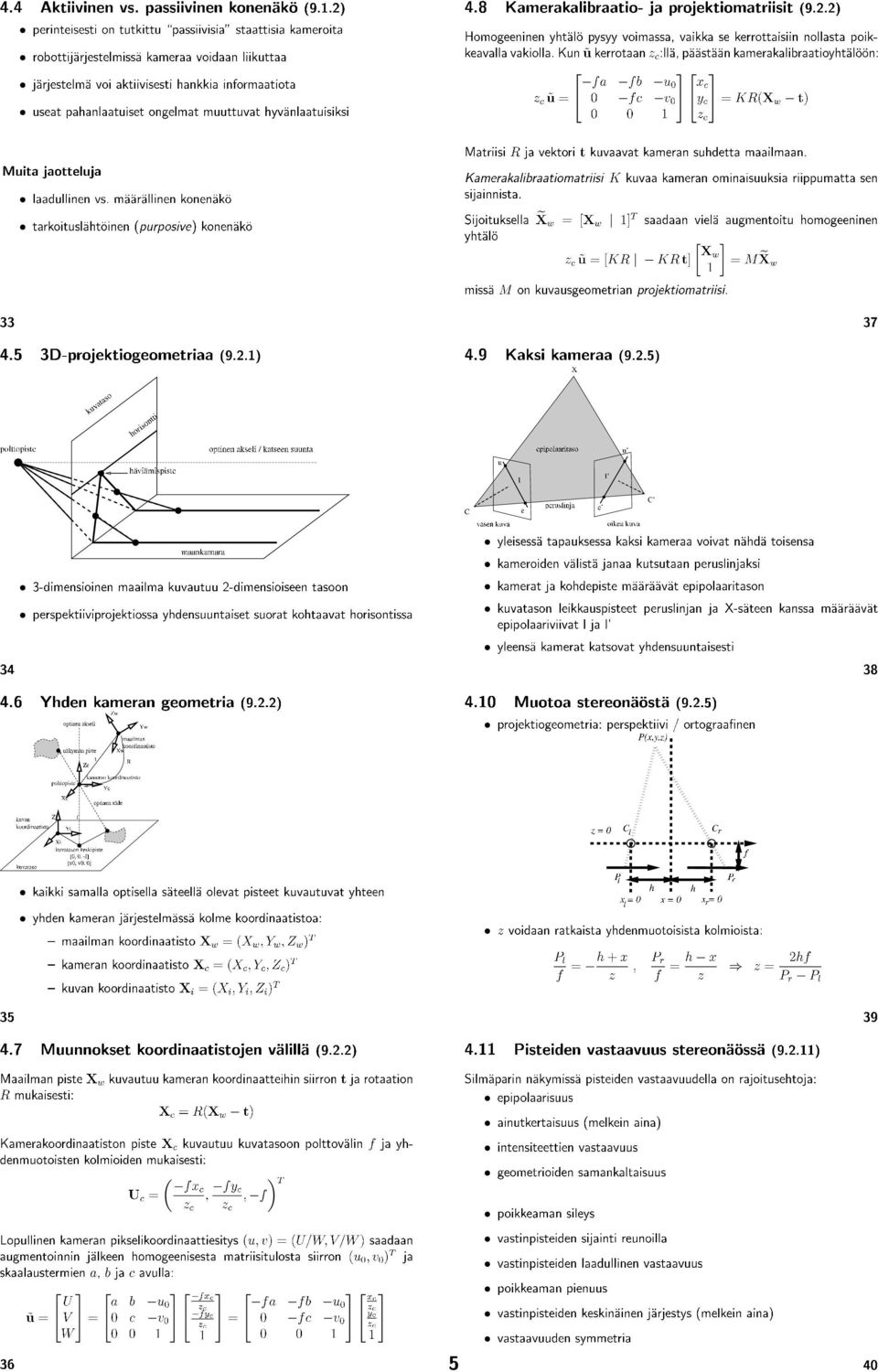
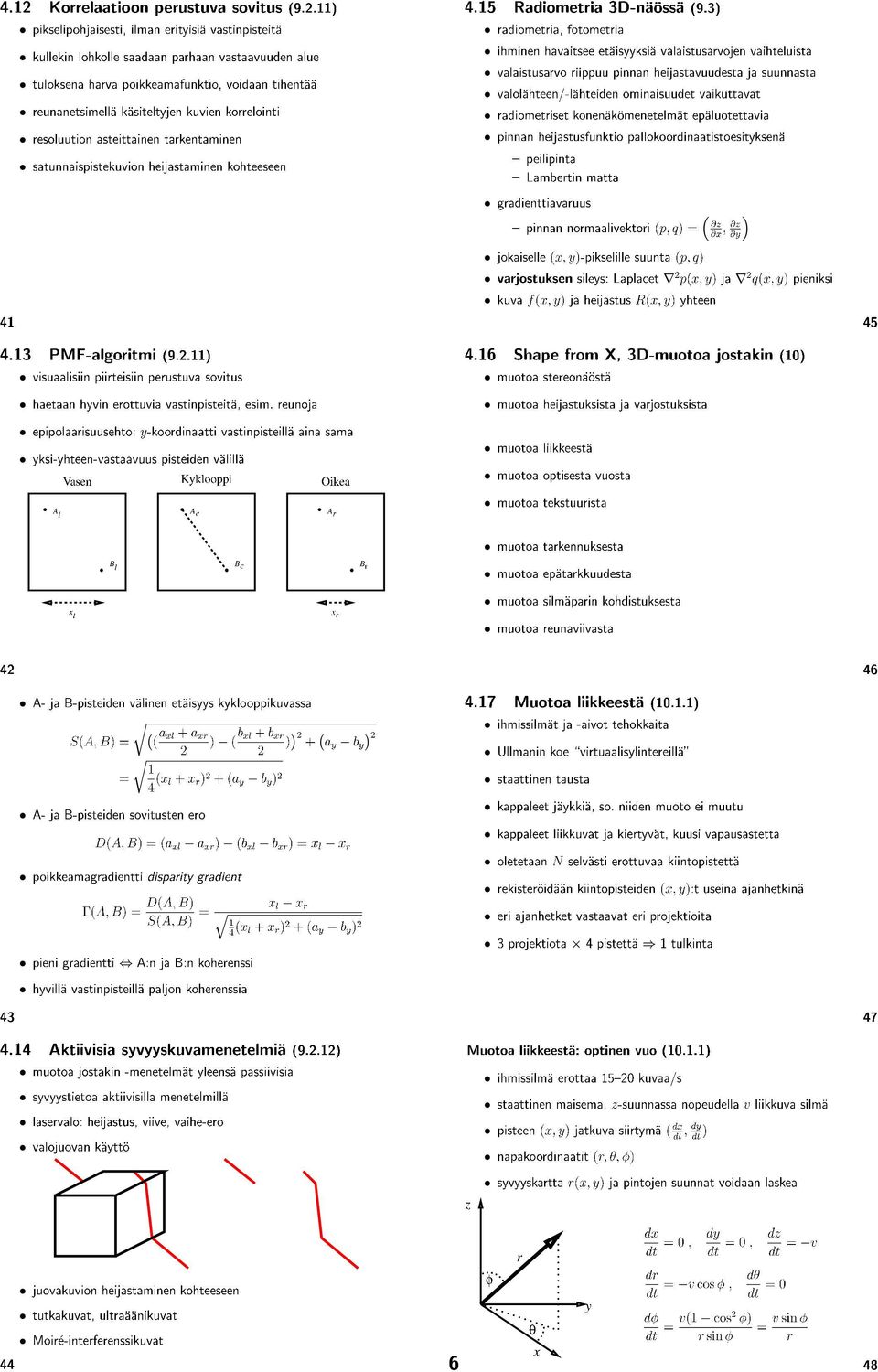
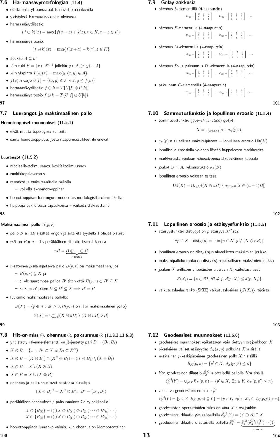
33 Exercise 1/07 33 T COMPUTER VISION, Exercise 1/07 1. The hexagonal grid is depicted in Fig. 1. The coordinates give the memory locations of grid elements. The six nearest neighbors of element (2,1) in Fig. 1 are N (2,1) {(3,0),(2,0),(1, 0),(1,1),(2, 2), (3,1)}. The nearest neighbors of each grid element are (i + 1,j 1),(i,j 1),(i 1,j 1),(i 1,j),(i,j + 1),(i + 1,j) if i is even, N (i,j) = (i + 1,j),(i,j 1),(i 1,j),(i 1,j + 1),(i,j + 1),(i + 1,j + 1) if i is odd. (1) (0, 0) (2, 0) (1, 0) (3, 0) (0, 1) (2, 1) (1, 1) (3, 1) (0, 2) (2, 2) (1, 2) (3, 2) Figure 1: Hexagonal grid in memory. The average for six nearest neighbors is calculated and substituted to each element, the image boundaries are not considered. This can be done by the following program: for(i=1;i<n-1;i=i+2) /* process odd-i elements */ for(j=1;j<n-1;j=j+1) ave[i][j] = (x[i][j] + x[i+1][j] + x[i][j-1] + x[i-1][j] + x[i-1][j+1] + x[i][j+1] + x[i+1][j+1])/7; for(i=2;i<n-1;i=i+2) /* process even-i elements */ for(j=1;j<n-1;j=j+1) ave[i][j] = (x[i][j] + x[i+1][j-1] + x[i][j-1] + x[i-1][j-1] + x[i-1][j] + x[i][j+1] + x[i+1][j])/7; Fig. 2 depicts distances in a hexagonal grid. Euclidian distances are calculated in a hexagonal grid from displacements d i and d j in directions i and j. d(p 1,p 2 ) = d 2 i + d2 j. (2) If i 1 i 2 is even, i.e. both elements are either in C e {c 0,c 2,c 4, } or in C o {c 1,c 3,c 5, }, the displacement d i is 3(i1 i 2 ) d i = (3) 2 and the displacement d j is simply d j = j 1 j 2. (4)

34 34 Exercise 1/07 c 0 c 1 c 2 c 3 (0, 0) (2, 0) i (0, 1) (1, 0) 1 1/2 3/2 j (0, 2) Figure 2: Distances in a hexagonal grid. When i 1 i 2 is odd, the displacement d i is obtained from Eq. 3 but displacement d j from Eq. 4 would be 0.5 units too large for even i 1 (i 1 C e ) and 0.5 units too small for an odd i 1 (i 1 C o ). Therefore, d j for an even i 1 is d j = j 1 j (5) and for an odd i 1 d j = j 1 j (6) Euclidean distances may be computed with the following program diff = j1 - j2; if (((i1 - i2) % 2)!= 0) { if ((i1%2) == 0) diff -= 0.5; else diff += 0.5; } dist = diff * diff; diff = i1 - i2; dist += 0.75 * diff * diff; dist = sqrt(dist); 2. Position-dependent brightness correction is represented in Sec. 4.1, pp The correction is made, for each image pixel (i), with the light and dark calibration targets, g l (i) and g d (i). For a linear degradation, the degraded image, f(i), is given by f(i) = k(i)g(i) + b(i) (7) The calibration values for k(i) and b(i) of each pixel are obtained from the equation pair { fl (i) = k(i)g l (i) + b(i) f d (i) = k(i)g d (i) + b(i). (8) The systematic brightness error can be suppressed by g(i) = f(i) b(i). (9) k(i)

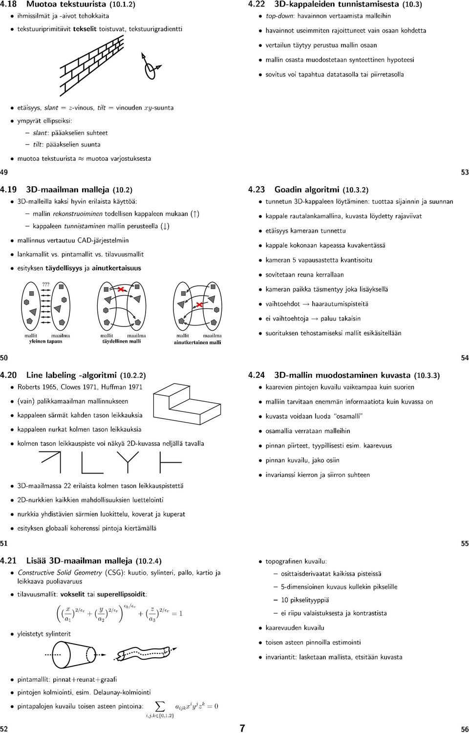
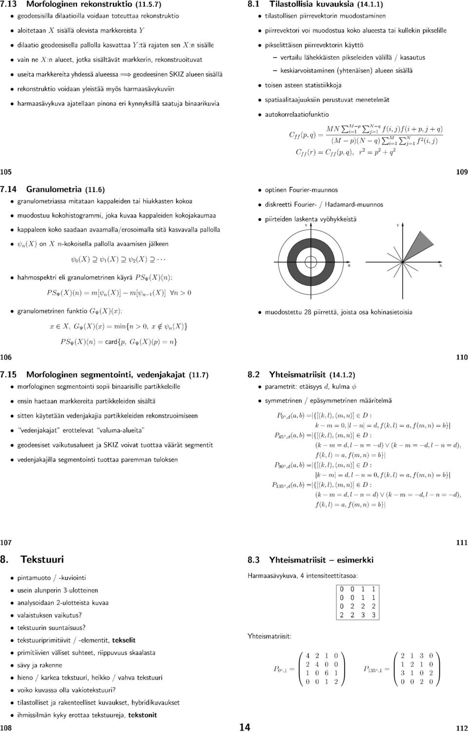
35 Exercise 1/07 35 e(x) n s θ i B(x) θ e da Figure 3: Radiometric image formation. 3. The radiometric image formation is depicted in Fig. 3. The following definitions are made: e(x) Incident surface irradiance, which is the power per unit area of radiant energy falling on a surface. It is measured in units of watts per square meter (W/m 2 ). B(x) Surface radiance, which is the power per unit foreshortened area emitted into a unit solid angle. It is measured in units of watts per square meter per steradian (W/m 2 /sr). Radiance can be a function of the viewing angle and the spectral wavelength and bandwidth. r(x) Surface reflectivity function (a.k.a. the reflectance, the reflection coefficient, or the bidirectional reflectance distribution function), which is the ratio of the radiant power per unit area per steradian reflected by the surface to the radiant power per unit area incident on the surface. It can be a function of the incident angle of the radiance, the viewing angle of the sensor, and the spectral wavelength and bandwidth. θ i Incidence angle. θ e Emittance angle. The incident surface irradiance e(x) is captured by an infinitesimal surface element da. The power is given by the projection e(x) dacos θ i. The amount of surface illumination seen by a viewer is given by B(x) dacos θ e. The surface reflectivity function relates these two quantities by the ratio r(x) = B(x)cos θ e e(x)cos θ i (10) In this case we want to calculate the surface radiance as seen from a certain angle θ e, i.e. the foreshortened B(x) cos θ e. Lets call this simply B e (x). Then we get: B e (x) = e(x)cos θ i r(x). (11) Lambertian surfaces have the property that under uniform illumination they look equally bright from any direction. The amount of light reflected from a unit area goes down as the cosine of the viewing angle, but the amount of area seen in any solid angle goes up as the reciprocal of the cosine of the viewing angle. Because we relate the perceived brightness to radiant power per solid angle, Lambertian surfaces seem to have the same brightness independent of viewing angle. This leads to the surface reflectivity function being constant for Lambertian surfaces, i.e. r(x) = r 0. This property is also sometimes given as the definition of a Lambertian surface.

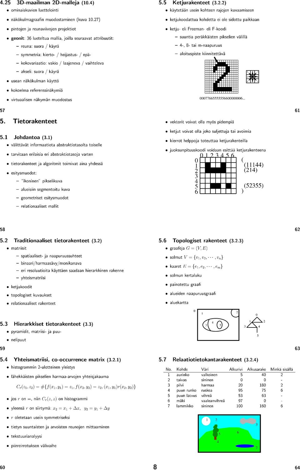
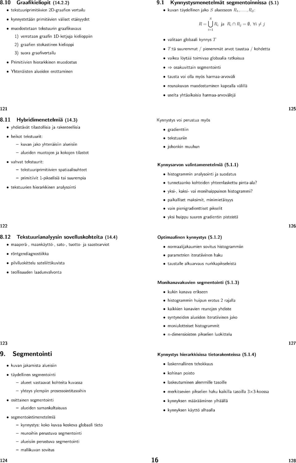
36 36 Exercise 1/07 n s = p l = 0 0 d θ i p i = x y Figure 4: A Lambertian plane illuminated by a point source of light. a) A Lambertian plane is illuminated by a point source of light at p l, Fig. 4. The reflectivity function r(p i ) of the plane is constant, r(p i ) = r 0. The irradiance e(p i ) varies inversely as the square of the distance from the illuminated surface to the source (law of inverse squares), e(p i ) = I 0 /d 2 s. B e (p i ) = e(p i )cos θ i r(p i ) = I 0 cos θ i r 0 d 2 s = I 0 r 0 p l p i 2 n s (p l p i ) n s p l p i = I 0 r 0 [0 0 1][ x y d] T (x 2 + y 2 + d 2 ) 3/2 = I 0 r 0 d (x 2 + y 2 + d 2 ) 3/2 (12) The brightest point on the plane is illuminated from normal direction (x = y = 0 B e (p i ) = I 0 r 0 /d 2 ) and around this point the brightness decreases concentrically with decreasing illumination angle. p i = n s = x y z p l = 0 0 d Figure 5: A Lambertian sphere illuminated by a point source of light. b) A Lambertian sphere is illuminated by a point source of light p l, Fig. 5. Assume that the sphere has a unit radius, i.e., x 2 + y 2 + z 2 = 1. [x y z][ x y d z] T B e (p i ) = I 0 r 0 (x 2 + y 2 + z 2 + d 2 2dz) 3/2 = I 0 r 0 x 2 y 2 z 2 + dz (d 2 2dz + 1) 3/2 = I 0r 0 (dz 1) (d 2 2dz + 1) 3/2 (13)

37 Exercise 1/07 37 The brightest point is illuminated from normal direction (z = 1 B e (p i ) = I 0 r 0 /(d 1) 2 ). The brightness reaches zero at z = 1/d where the light hits the sphere tangentially. 4. Two point sources of light illuminate a Lambertian plane, Fig. 6. The irradiance is e(p i ) = I 0 /d 2 s. The reflectivity function r(p i ) = r 0 is constant. The surface radiance at point p i = [x y 0] T is then B e (p i ) = I 0 r 0 ( cos θa i d 2 A + cos θb i d 2 B ( ns (p A l p i ) ) = I 0 r 0 n s p A l p i 3 + n s (p B ) l p i ) n s p B l p i 3 ( ) [0 0 1][( e x) ( y) d] T [0 0 1][(e x) ( y) d]t = I 0 r 0 ((e + x) 2 + y 2 + d 2 ) 3/2 + ((e x) 2 + y 2 + d 2 ) 3/2 ( ) d = I 0 r 0 ((e + x) 2 + y 2 + d 2 ) 3/2 + d ((e x) 2 + y 2 + d 2 ) 3/2 The radiance B e (p i ) is a sum of two radiances decreasing concentrically around the brightest point. The plane has two radiance maxima, at p i = [ e 0 0] T and p i = [e 0 0] T. The isoradiance curves on the plane are depicted in Fig. 7 (e = 1). (14) A B θ A i θ B i Figure 6: A Lambertian plane illuminated by two point sources of light Figure 7: The variation of luminance at illumination by two point sources.

38 38 Exercise 2/07 T TIETOKONENÄKÖ, Harjoitus 2/07 Harjoitusten tarkoitus Harjoitusten tarkoituksena on tutustua kamerakalibraatioon, stereonäköön ja pintojen mallintamiseen. 1. Määrää kameran kalibraatioparametrit aktiiviselle ja passiiviselle kameralle oheisen taulukon perusteella. Käytä yhdeksää pistettä: 1, 3, 4, 5, 6, 8, 9, 10, 11. Laita a 34 = 1. Object-centered Active camera Passive camera coordinates Point# coordinates coordinates (global, inches) x a y a x i y i x 0 y 0 z ,72 1, ,05 0, ,64 3, ,76 5, ,22 4, ,57 0, ,58 0 3, ,16 2,84 2. Oletetaan kaksisilmäisen olion silmien väliksi h = 100mm ja silmien polttoväliksi f = 50mm. Piirrä x i -koordinaattien erotus (disparity) etäisyyden funktiona. Mikä on silmäparin käyttökelpoinen toiminta-alue etäisyyden arvioinnissa, kun silmien erotuskyky on 50 viivaparia/mm? 3. (a) Piirrä Delaunay triangulaatio oheisille datapisteille. (b) Muodosta Voronoi diagrammi käyttäen hyväksesi edellisen kohdan tulosta. (c) Muodosta datapisteiden konveksi peite (convex hull)

39 Exercise 2/07 39 T COMPUTER VISION, Exercise 2/07 Motivation The purpose of this exercise is to be acquainted with the camera calibration, stereo vision, and surface modeling. 1. Determine the calibration parameters for the active and passive cameras using these nine data points: 1, 3, 4, 5, 6, 8, 9, 10, 11. Set a 34 = 1. Object-centered Active camera Passive camera coordinates Point# coordinates coordinates (global, inches) x a y a x i y i x 0 y 0 z ,72 1, ,05 0, ,64 3, ,76 5, ,22 4, ,57 0, ,58 0 3, ,16 2,84 2. In a binocular animal vision system, assume a separation distance h = 100mm and a focal length of an eye f = 50mm. Make a plot of the disparity as a function of distance. If the resolution of each eye is on order of 50 line pairs/mm, what is the useful range of the binocular system? 3. (a) Draw the Delaunay triangulation to the given datapoints. (b) Construct the Voronoi diagram using the result from the previous item. (c) Construct the convex hull of the given datapoints

40 40 Exercise 2/07 T COMPUTER VISION, Exercise 2/07 1. Camera calibration is an essential stage in the utilization of a stereo imaging system. The relationship between pixel coordinates of 2-D image p i = [x i y i ] T and 3-D object p o = [x o y o z o ] T must be determined. The relationship is nonlinear and therefore difficult to analyze. y p i = x i y i 0 f = 0 0 f x z p 0 = x 0 y 0 z 0 Figure 1: Pinpoint camera model. For instance, in the simple pinpoint camera model the relationship is given by 0 0 f x i y i 0 f p i = k(p 0 f) = (1) = k [ xi y i x o y o z o ] [ = 0 0 f f f z o x o f f z o y o ] x i y i = kx o = ky o k = f z o f It is often convenient to linearize Eq. 3. This can be accomplished easily by using homogeneous coordinates. A vector is transformed to homogeneous coordinates simply by expanding it by a unity element. Calculations are performed just as in conventional matrix algebra. When transforming back to the conventional coordinate system, the vector is scaled by the value of the additional coordinate. Thus, the division operation can be regarded as implicitly implemented with the additional coordinate, value of which generally changes during calculations but still serves as a floating scaling factor: [ x y ] = The coordinates of a given image point are [ xi y i ] = x i y i 1 x y 1 f f z o x o f f z o y o 1 wx wy w (2) (3) (4) fx o fy o f z o. (5)

41 Exercise 2/07 41 The rightmost term in Eq. 5 can be expressed in matrix form as x fx o f o fy o = 0 f 0 0 y o z f z o f o. (6) 1 Thus, the (pinpoint) camera model can be expressed as p i = Ap o, (7) where the image coordinates are denoted by p i = [w i x i w i y i w i ] T, object coordinates by p o = [w o x o w o y o w o z o w o ] T and the imaging system (lenses etc.) by matrix A. The pinpoint camera model, that appears above as the simplicity of A, is not useful for real sensor systems which require more complex transforms. During camera calibration, the elements in such transform matrix A are estimated by studying sample object coordinates and resulting image points. If the matrix P o represents a set of object coordinates, the corresponding image points are obtained by P i = AP o. In practice, the imaging system contains (slight) nonlinearies and the measurements of object and image points contain errors. In other words, there is no exact solution for the linear model represented by A. An approximation of A could be achieved by A = P i P + o (cf. definition of pseudoinverse below), but a more sophisticated method is presented in R. J. Schalkoff: Digital Image Processing and Computer Vision, pp (see also the course book Sec p. 455): Eq. 7 is expressed with homogeneous coordinates as w i x i w i y i w i = a 11 a 12 a 13 a 14 a 21 a 22 a 23 a 24 a 31 a 32 a 33 a 34 x o y o z o 1. (8) Letting a 34 = 1 in the homogeneous representation and expanding the matrix product yields w i x i = x o a 11 + y o a 12 + z o a 13 + a 14 w i y i = x o a 21 + y o a 22 + z o a 23 + a 24 w i = x o a 31 + y o a 32 + z o a { xi = x o a 11 + y o a 12 + z o a 13 + a 14 x i x o a 31 x i y o a 32 x i z o a 33 y i = x o a 21 + y o a 22 + z o a 23 + a 24 y i x o a 31 y i y o a 32 y i z o a 33 (9) For each of the N image-object coordinate pairs there are two equations, written in matrix product d = Qa, where d = [x 1 i x N i yi 1 yi N]T, a = [a 11 a 12 a 13 a 14 a 21 a 22 a 23 a 24 a 31 a 32 a 33 ] T, and x 1 o yo 1 zo x 1 i x1 o x 1 i y1 o x 1 i z1 o x N o yo N zo N x N i Q = xn o x N i yn o x N i zn o x 1 o yo 1 zo 1 1 yi 1 x1 o yi 1y1 o yi 1z1 o x N o yo N zo N 1 yi NxN o yi NyN o yi NzN o There is no solution for a = Q 1 d, because Q is not a square matrix. Therefore, vector a is searched for, which realizes the equation as well as possible, d = Qa + e, where e is an error term. The error can be minimized with the minimum squared error method. Find such a which minimizes the squared error e T e = (d Qa ) T (d Qa ) = d T d a T Q T d d T Qa + a T Q T Qa. (10)

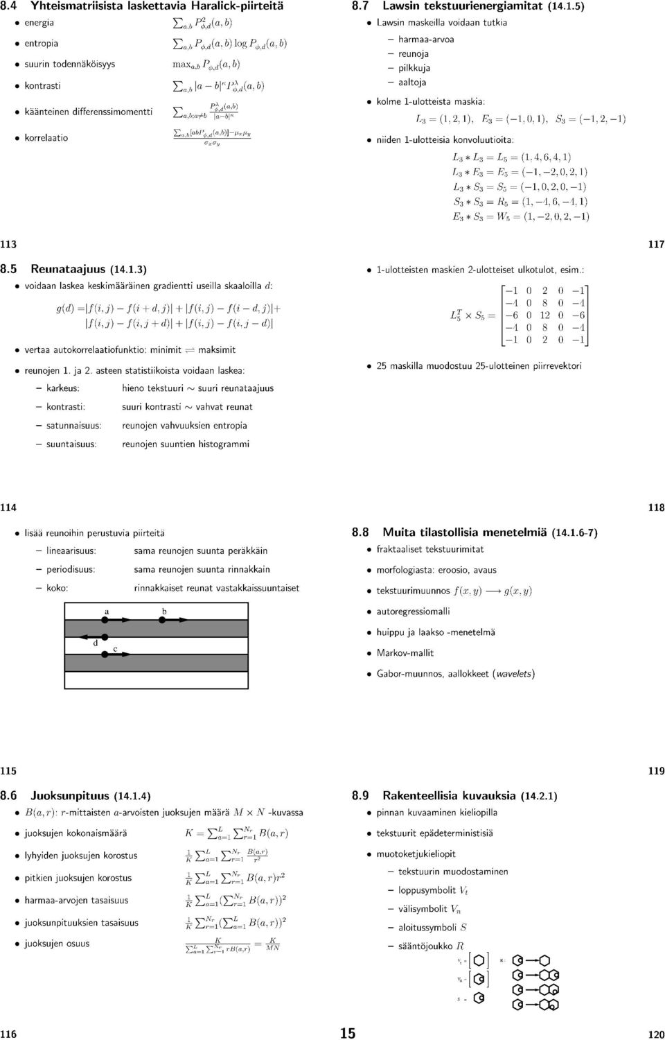
42 42 Exercise 2/07 Differentiation with respect to a and setting the result equal to zero gives de T e da = 2Q T d + 2Q T Qa = 0 Q T Qa = Q T d a = (Q T Q) 1 Q T d = Q + d (11) Matrix Q + is the pseudoinverse of Q. For the calibration of the active and passive camera the values calculated for Q and d are substituted into the pseudoinverse equation. This may be done with MATLAB. Xo = [ ] ; Yo = [ ] ; Zo = [ ] ; Xi = [ ] ; Yi = [ ] ; zer = [ ] ; one = [ ] ; q1 = [Xo Yo Zo one zer zer zer zer -Xi.*Xo -Xi.*Yo -Xi.*Zo]; q2 = [zer zer zer zer Xo Yo Zo one -Yi.*Xo -Yi.*Yo -Yi.*Zo]; Q = [q1 ; q2]; d = [Xi ; Yi]; Calibration parameters for the active camera a = inv(q *Q) * Q * d Xi = [ ] ; Yi = [ ] ; q1 = [Xo Yo Zo one zer zer zer zer -Xi.*Xo -Xi.*Yo -Xi.*Zo]; q2 = [zer zer zer zer Xo Yo Zo one -Yi.*Xo -Yi.*Yo -Yi.*Zo]; Q = [q1 ; q2]; d = [Xi ; Yi]; Calibration parameters for the passive camera a = inv(q *Q) * Q * d Calibration parameters for the active camera: , , , , , , , , , , Calibration parameters for the passive camera: , , , , , , , , , Binocular imaging geometry is represented in Sec pp A point in a 3-dimensional scene, P(x,y,z), is projected onto the retinas of two eyes with 2h separation, Fig. 2. The projection point on the left retina is x l and on the right x r. In the depicted case, x l is negative and x r is positive. Disparity is the difference x r x l and it is always non-negative.

43 Exercise 2/07 43 P(x, y, z) z = 0 c l c r f x l h h x r x l = 0 x = 0 x r = 0 Figure 2: Stereo vision geometry (Sonka et al. 1993). According to the geometry of similar triangles Distance x is eliminated: Disparity x r x l is given by x l f = h x l + x z + f x = hf + x lz f and x r f = h + x r x. (12) z + f = hf x rz. (13) f z(x r x l ) = 2hf x r x l = 2hf z. (14) Resolution of retinal images is 50 lines/mm, separation of the eyes is 100, and focal length is 50 mm. Disparity is plotted as the function of object distance z in Fig. 3. The maximum object distance for a stereo image is 100 mm 50 mm = 250 m. (1/50) mm 3. a) In Delaunay triangulation the task is to find triangles that cover all data points in such a way that the circumcircle of any one triangle contains only the three points that are vertices of that particular triangle. Let us start from the left edge on the given image. If we connect the first three points and draw a circle around them (Figure (a)), we notice that no other point lies inside the circle and thus our triangle is a valid one. Then we add a new point and form a new triangle (Figure (b). When we now draw a circle around our new triangle, the point marked with an arrow lies inside the circle, and thus our new triangle is not a valid one and we remove it. We then select another point, form a new triangle, test it by drawing a circle around it and so on (Figure (c)).

44 44 Exercise 2/ Disparity/mm Distance/m Figure 3: Disparity as a function of object distance. Finally we obtain the final Delaunay triangulation (Figure (d)). Notice that our solution is unique only if no more than three points lie on one circle! (a) (b) (c) (d) b) The Voronoi diagram on the given set of points is a set of convex polyhedra (or polygons in 2D space) that covers the whole space. Each given point M i has one polyhedron V i, and each polyhedron V i covers all points in the space that are closer to the point M i than to any other given point.

45 Exercise 2/07 45 The Voronoi diagram can be constructed using the Delaunay triangulation. The midpoints of the sides of the triangles are recorded. The normal vectors are drawn to each triangle side through its midpoint (to both directions). The crossings of these normal vectors are calculated and convex polygons are formed. These polygons form the Voronoi diagram. In the next figure the Voronoi diagram is drawn with solid lines and the Delaunay triangulation with dotted lines. Polygons that contain a point at infinity are not drawn c) The convex hull is obtained very easily, since it corresponds to the boundary of the set of points covered by triangles that were obtained by the Delaunay triangulation in a). In the next figure the convex hull is drawn with solid lines over the Delaunay triangulation (the dotted lines)

46 46 Exercise 3/07 T TIETOKONENÄKÖ, Harjoitus 3/07 Harjoitusten tarkoitus Harjoitusten tarkoituksena on tutustua tietorakenteisiin sekä tavallisimpiin digitaalisille kuville tehtäviin geometrisiin muunnoksiin. 1. Näytä miten hierarkinen etsintä ja sovittaminen toimivat oheisessa tapauksessa. TEMPLATE IMAGE Kehitä algoritmi, joka etsii kahden nelipuina esitetyn alueen leikkauksen ja muodostaa tästä nelipuun. Anna esimerkki! 3. Alla on annettu kaksi viivakuvaa (binäärikuvaa). Valitse sopivat kontrolllipisteet ja muunna kuvan 2 koordinaatisto kuvan 1 koordinaatistoon käyttäen (a) affine-muunnosta, (b) 2D polynomista kiertoa (warp), kun N = 2. Scale: 1 tick = 10 units y y x Image 1 x Image 2 4. (a) Näytä analyyttisiä menetelmiä ja esimerkkejä käyttäen miksi bilineaarinen muunnos, f(x,y ) = (1 a)(1 b)f(x,y)+a(1 b)f(x+1,y)+(1 a)bf(x,y+1)+abf(x+1,y+1), ei välttämättä ole yhtenevä kontrollipisteiden intensiteettien määrittämän tason kanssa (eli ei välttämättä sovita tasoa kontrollipisteiden välille). (b) Millä ehdoilla muunnoksen antama piste ja kontrollipisteiden intensiteettien muodostama taso ovat yhtenevät?

47 Exercise 3/07 47 T COMPUTER VISION, Exercise 3/07 Motivation The purpose of this exercise is to be acquainted with data structures and the most usual geometric corrections. 1. Demonstrate how hierarchical search and matching work on the given example. TEMPLATE IMAGE Suggest an algorithm that can find an intersection between two regions represented as quadtrees. The intersection should be represented as a quadtree. Give an example! 3. Given the two binary images (below), choose appropriate control points and correct the coordinate system of the image 2 to the coordinate system of the image 1 using (a) an affine transform, (b) a 2D polynomial warp of 2nd order (N = 2). Scale: 1 tick = 10 units y y x Image 1 x Image 2 4. (a) Using both analytical justification as well as graphical examples, show why the bilinear interpolation technique, f(x,y ) = (1 a)(1 b)f(x,y)+a(1 b)f(x+1,y)+(1 a)bf(x,y+1)+abf(x+1,y+1), does not necessarily fit a plane to the interpolated intensity region. (b) What are the conditions on the local image intensities such that the bilinear interpolation technique results in fitting a plane to the image intensities?

48 48 Exercise 3/07 T COMPUTER VISION, Exercise 3/07 1. Scene matching is represented in Sec. 5.4, pp Anil K. Jain represented hierarchical search in his book Fundamentals of Digital Image Processing, p. 407, as follows: If the observed image is very large, we may first search a low-resolution-reduced copy using a likewise reduced copy of the template. If multiple matches occur, then the regions represented by these locations are searched using higher-resolution copies to further refine and reduce the search area. Thus the full-resolution region searched can be a small fraction of the total area. This method of coarse-fine search is also logarithmically efficient. A coarse search is performed by reducing both the image and the template and by matching the reduced template to the image. The reductions are accomplished by replacing every 2 2 neighborhood by its average. Values are rounded to the nearest integer. The reduced template is h r (i,j) = The reduced image is f r (u,v) = Squared distance of the template from the image blocks yields a measure for their similarity C(u,v) = (i,i) V [f(i + u,j + v) h(i,j)] 2 = (1) The best-matching point, indicated in bold in the distance array, is suggestive for further evalution. A finer search is done by matching the original template to this site in the original image The smallest squared distance for the template match, 91, was obtained when the left upper corner of the template was at position (2,0) in the image....

49 Exercise 3/ Quadtrees are represented in Sec , pp Two sample images A and B, their intersection, and the corresponding quadtrees are depicted in Fig. 1. The algorithm starts from the root node by processing its child nodes from left to right and by creating nodes in the intersection tree according to the following cases 1. Create a black leaf node if both counterpoint nodes are black leaf nodes. 2. Create a white leaf node if either or both counterpoint nodes are white leaf nodes. 3. Create a parent node if counterpoint nodes are a parent node, denoted by n, and a black leaf node. The child nodes of the parent node n are copied to the intersection tree. 4. If both counterpoint nodes are parent nodes then create a parent node and process iteratively the child nodes. If all child nodes result in white leaf nodes then replace the parent node with a white leaf node. A B A B Quadtree of A Quadtree of B Quadtree of A B Figure 1: Two sample images, their intersection, and the quadtrees.

50 50 Exercise 3/07 3. a) Affine transformations (Sec p. 64) can be expressed in homogeneous coordinates by matrix product p = Ap, where p = x y 1, p = x y 1,and A = a 11 a 12 a 13 a 21 a 22 a (2) The matrix A is a combination of scaling A sc, skewing A sw, rotation A rt, and translation A tr, A = A sc A sw A rt A tr Scaling Skewing Original Rotation Translation A sc = A rt = s x s y cos θ sinθ 0 sinθ cos θ , A sw = 1 tan φ ,and A tr =, 1 0 t x 0 1 t y (3) The order of different transformations is significant. Rotation followed by translation does not necessarily give the same result as translation followed by rotation. Control points p 1, p 2,, p N and their counterpoints p 1, p 2,, p N are selected to determine A. P 3 N = A 3 3P 3 N, P = x 1 x 2 x N y 1 y 2 y N 1 1 1, P = x 1 x 2 x N y 1 y 2 y N (4) Six elements in matrix A are unknown. Therefore, three control points must be selected to solve for A = P P 1. For instance, the following points may be chosen P = [ ; ; 1 1 1]; Pc = [ ; ; 1 1 1]; A = Pc * inv(p) A =

51 Exercise 3/07 51 b) In the previous exercise, affine transforms were used for representation of geometric distortion functions. In this exercise, the functions are approximated by Nth order 2-D polynomials, yielding the so-called polynomial warp model. Notice that no assumptions about the viewing geometry or about the character of geometric distortion are necessary. The degree of the 2-D polynomial is often selected empirically, or it is restricted by the number of available control points. The polynomial warp relationship is determined by x = N N ˆk ijx 1 i y j (5) i=0 j=0 An example of polynomial warp: N N y = ˆk ij 2 xi y j. (6) i=0 j= x = x x2 1 y = y y x xy Warp ˆk 1,2 In our case, N is 2. The 18 coefficients ij of the 2-D polynomial are estimated with two estimation equations from each control point. Therefore, at least nine control points are required. The transformation is given by p = Kw, where Matrix K 2 9 = P 2 9 W 1 9 9, where p = [x y ] T, [ ] ˆk1 K = 00 ˆk1 10 ˆk1 01 ˆk1 22 ˆk 01 2, and ˆk2 22 ˆk 2 00 [ x P = 1 x N y 1 y N ˆk 2 10 w = [1 x y xy x 2 y 2 x 2 y xy 2 x 2 y 2 ] T. (7) ] and W = The following points may be chosen, for instance Px = [ ] ; Py = [ ] ; Pc = [ ; ]; one = [ ] ; W =[one Px Py Px.*Py Px.*Px Py.*Py Px.*Px.*Py... Px.*Py.*Py Px.*Px.*Py.*Py] ; K = Pc * inv(w) 1 1 x 1 x N.. x 2 1 y2 1 x 2 N y2 N.

52 52 Exercise 3/07 f(x, y) y b a x x (1, 1) y y (a) (b) (c) x Figure 2: Bilinear interpolation K = 4. Columns 1 through Columns 7 through a) Bilinear interpolation is represented as linear interpolation in Sec , p. 67. Assume that values of function f are known at points (0,0), (0,1), (1,0), and (1,1), Fig. 2. Bilinear interpolation yields the values of f(a, b), a [0, 1] and b [0, 1] f(a,b) = (1 a)(1 b)f(0,0) +a(1 b)f(1,0) +(1 a)bf(0,1) +abf(1,1) (8) The Eq. 8 is a plane equation if it has the form f(a,b) = f 0 + f 1 a + f 2 b, i.e., the equation f(a,b) = f(0,0) + [f(1,0) f(0,0)]a + [f(0,1) f(0,0)]b +[f(0,0) f(1,0) f(0,1) + f(1,1)]ab (9) is a plane equation only if the factor of ab is equal to zero. For instance, if f(0,0) = f(1,0) = f(0,1) = 1 and f(1,1) = 0, then f(a,b) = 1 ab, which is not a plane, Fig. 2 (b). On the other hand, if f(0,0) = f(1,0) = 1 and f(0,1) = f(1,1) = 0, then f(a,b) = 1 b, which is a plane, Fig. 2 (c) Bilinearity: linear performance if either variable is fixed!

53 Exercise 3/07 53 b) The Eq. 9 is a plane equation if f(0,0) + f(1,1) = f(1,0) + f(0,1), (10) i.e., when the control points f(0,0), f(1,1), f(1,0), and f(0,1) are in the same plane.

54 54 Exercise 4/07 T TIETOKONENÄKÖ, Harjoitus 4/07 Harjoitusten tarkoitus Harjoitusten tarkoituksena on palauttaa mieliin keskeisimmät reunanhaku- ja kuvanparannusmenetelmät. 1. Sovella seuraavia reunanetsintämenetelmiä oheiseen kuvaan: (a) Robertsin gradientti (b) Sobelin menetelmä (c) Frein ja Chenin menetelmä Näytä esimerkillä, että epäsymmetriseen ikkunaan perustuva mediaanisuodatus saattaa siirtää reunan paikkaa. 3. Ehdota reunanetsintämenetelmä, jota voidaan käyttää sekä voluumikuvissa (3D) että useampikanavaisissa satelliittikuvissa. 4. Oletetaan, että muuttujan x jakauma on f(x), joka poikkeaa nollasta välillä [a, b]. Määritä muunnos y = g(x) siten, että y:n jakauma on tasainen välillä [0,c]. Kehitä tämän tuloksen perusteella algoritmi, jolla kuvan kirkkausarvojen histogrammi voidaan tasoittaa.

55 Exercise 4/07 55 T COMPUTER VISION, Exercise 4/07 Motivation The purpose of this exercise is to brush up the most central edge detection and image enhancement methods. 1. Test the following edge detection algorithms for the given image: (a) Roberts operator (b) Sobel operator (c) Frein and Chen gradient masks Show that median filtering based on an unsymmetrical neighbourhood may move the location of an edge. 3. Suggest an edge detection algorithm that can be used for volume images (3D) and for multispectral satellite images. 4. Assume a non-zero intensity distribution f(x), {x [a,b]}, in an image. Define a transform y = g(x) so that the distribution of y will be even in the range [0,c]. Derive an algorithm for histogram equalization based on that transform.

56 56 Exercise 4/07 T COMPUTER VISION, Exercise 4/07 1. Edge detecting spatial filters are described in Sec , pp The convolution masks for Roberts operator are 1 0 h 1 : 0 1 and h : 1 0. Sobel operator defines two convolution masks suitable for the detection of horizontal and vertical edges: h 1 : and h 2 : Frei and Chen used a set of nine orthogonal masks to detect edges and lines, or neighborhoods without edges and lines. Four of the nine masks are suitable for edge detection: h 1 : , h 2 : ,h 3 : , and h 4 : The output of mask h k is given by f k (i,j) = (m,n) R h k (i m,j n)g(m,n), where g(m,n) is the image pixel and R defines the local neighborhood of the pixel f k (i,j). The L 2 norm of the mask outputs, k f2 k, was used to describe edginess in the response images shown below. Sometimes, the simpler L 1 norm ( k f k ) is used as an approximation altough the systematic error increases with dimension Original Roberts Sobel Frei & Chen

57 Exercise 4/ Median smoothing (pp ) ranks local pixel intensities and replaces the gray level of each pixel by the median of the gray levels in a neighborhood of that pixel. Define the support for a nonsymmetric median smoothing mask as As shown by the following example, a nonsymmetric median filter may shift edge locations. Original image Filtered image A symmetric median smoothing mask, e.g., preserves edge locations. 3. Some methods for finding edges in multispectral images are described in Sec , p. 94. The edge detector of Cervenka and Charvat, Eq. (4.68) in the textbook, is not appropriate for 3-D images because it does not take the gradient in z-direction into account. In 3-D data object boundaries are surfaces; edge elements in two dimensions become surface elements in three dimensions. The two-dimensional image gradient, when generalized to three dimensions, is the local surface normal. For a given volume image f(x,y,z), the gradient of f is the vector defined by f = f x i + f y j + f z k, where i = [1 0 0] T, j = [0 1 0] T, and k = [0 0 1] T are the unit vectors. A simple measure of 3-D edginess is the magnitude of the surface gradient computed from differences approximating the first derivatives in the directions of x, y, and z: M = ( x f) 2 + ( y f) 2 + ( z f) 2, where x f = f(x + 1,y,z) f(x,y,z), y f = f(x,y + 1,z) f(x,y,z), z f = f(x,y,z + 1) f(x,y,z). This method is applied to multispectral images by forming the z-component using the n spectral bands f 0 (x,y), f 1 (x,y),, f n 1 (x,y): f(x,y,z) = f z (x,y) The brightness difference of the same pixel in two adjacent spectral bands, z f, is very informative. (An example: The AVHRR instrument of NOAA weather satellites has five spectral channels. Some object characteristics are emphasized by differences between adjacent spectral bands, for example: The difference f 1 (x,y) f 0 (x,y) serves the detection of vegetation and snow,and discrimination between land and sea. The difference f 3 (x,y) f 2 (x,y) serves the detection of cirrus clouds and the discrimination between watercloud and surface, and between snow and cloud. The difference f 4 (x,y) f 3 (x,y) serves the detection of precipitation clouds.)

58 58 Exercise 4/07 F x(x) 1 F y(y) 1 d k d k a x k a. b x y k b. c y Figure 1: Distribution function of some f x (x) (a.) and distribution function of constant density f y (y) (b.). 4. Histogram equalization is described in Sec , pp in the textbook. A function y = g(x) is determined for transforming the non-uniform density function of x, f x (x), into the constant density function of y, f y (y) = k. A cumulative distribution function of some f x (x), F x (x), is depicted in Fig. 1.a. A distribution function of constant density f y (y), F y (y), is depicted in Fig. 1.b. The intensity transform y = g(x) should be found which maps a value of x to a value of y so that F y (y) = F x (x). Solve for y: F y (y) = y 0 f y (y)dy = y 0 kdy = ky = y = 1 k x a x a x a x The normalization coefficient k can be determined from Therefore, F y (c) = c 0 y = g(x) = c f x (x)dx = F x (x). f x (x)dx f x (x)dx a f x (x)dx. f y (y)dy = 1 kc = 1 k = 1 c. x The histogram equalization algorithm is as follows: a f x (x)dx = cf x (x). 1. Compute the histogram of intensity levels f x (x) in the input image. 2. Sum f x (x) to obtain the distribution function F x (x). 3. Use F x (x) as the intensity transformation function g(x); that is, y = cf x (x), where c is the largest intensity level in the transformed histogram.

59 Exercise 5/07 59 T TIETOKONENÄKÖ, Harjoitus 5/07 Harjoitusten tarkoitus Harjoitusten tarkoituksena on tutustua morfologiseen suodatukseen. 1. Todista seuraavat dilaation ominaisuudet (kirjan sivu 564): (a) X B = B X (b) X (B D) = (X B) D (c) X B = b B X b (d) X h B = (X B) h 2. Miten saat oheisen kuvan kohteen siistityksi tunnistusta varten käyttäen morfologisia suotimia? (Kuvassa olevan nollan reunaviiva tulisi saada yhtenäiseksi.) Laske oheisten kuvien kohteiden rungot (luurangot) käyttäen kirjan algoritmia 6.8 (s. 267) sekä morphologisia operaatioita

60 60 Exercise 5/07 T COMPUTER VISION, Exercise 5/07 Motivation The purpose of this exercise is to be acquainted with morphological filtering. 1. Proof the following properties of dilation (page 564 in the textbook): (a) X B = B X (b) X (B D) = (X B) D (c) X B = b B X b (d) X h B = (X B) h 2. How can the given object be cleaned up by using morphological operations? (The outline of the zero in the image should be closed.) Skeletonize the objects in the given images by using the algorithm 6.8 (p. 267) in the textbook and the morphological operations

61 Exercise 5/07 61 T COMPUTER VISION, Exercise 5/07 1. We will need the following definitions of dilation and translation. The dilation of the point set X by the structuring element B is defined as X B = {p E 2 : p = x + b,x X and b B}. The translation of the point set X by the vector h is defined by X h = {p E 2 : p = x + h for some x X}. a) Proof that dilation is commutative, X B = B X. Proof: X B = {p p = x + b for some x X,b B} = {p p = b + x for some x X,b B} = B X b) Proof that dilation is associative, X (B D) = (X B) D. Proof: p X (B D) if and only if there exists x X, b B, and d D such that p = x + (b + d). p (X B) D if and only if there exists x X, b B, and d D such that p = (x + b) + d. But x+(b+d) = (x+b)+d since addition is associative. Therefore, X (B D) = (X B) D. c) Proof that dilation may also be expressed as a union of shifted point sets, X B = b B X b. Proof: Suppose that p X B. Then for some x X and b B, p = x + b. Hence, p (X) b and therefore p b B X b. Suppose p b B X b. Then for some b B, p (X) b. But p (X) b implies there exists an x X such that p = x+b. Now by definition of dilation, x X and b B, and p = x+b imply p X B. d) Proof that dilation is invariant to translation, X h B = (X B) h. Proof: y X h B if and only if for some z X h and b B, y = z + b. But z X h if and only if z = x + h for some x X. Hence, y = (x + h) + b = (x + b) + h. Now by definition of dilation and translation y (X B) h.

62 62 Exercise 5/07 2. The morphological operation closing (Sec , pp ) is used to close the outline of the zero (or rectangle) in the given image X. The image is plotted in Fig. 1 a), with 0 as white (background) and 1 as black (the object). Closing is dilation followed by erosion. Dilation is defined as Erosion is defined as Closing is defined as X B = {p E 2 : p = x + b,x X and b B}. X B = {p E 2 : p + b X for every b B}. X B = (X B) B. Fig. 1 b) - f) shows results for closing with different structural elements. The first column shows the structural element, x marks the local origin (representative point), black squares mark points belonging to the element. The second column shows the result after dilation, the third column the result after eroding the dilated image, i.e. the final closing result. In this case the d) element gives the cleanest image with a closed outline. 3. Skeletonizing with thinning The skeleton can be obtained with the thinning algorithm 6.8, p The first image The set of region pixels R for the first image is R = Define H i (R) as the inner boundary of R (border of image) and H o (R) as the outer boundary of R (border of background). Let S(R) be a set of pixels from region R which have all their neighbors in 8-connectivity either from the inner boundary H i (R) or from the background. Assign R old = R. Construct a region R new which is the result of one-step thinning as follows R new = S(R old ) [R old H i (R old )] [H o (S(R old )) R old ]. The sets S(R old ) and H o (S(R old )) R old are empty. R new = R old H i (R old ) = The new iteration gives the same image R new. Therefore, R new is a set of skeleton pixels of the region R.

63 Exercise 5/07 63 a) b) c) d) e) f) Figure 1: Closing with different structural elements (b-f). The original is shown in (a).

64 64 Exercise 5/07 The second image The set of region pixels R for the second image is R = Assign R old = R. The sets S(R old ) and H o (S(R old )) R old are empty. Therefore, the region R new = R old H i (R old ). R new = Assign R old = R new and continue. S(R old ) = R old H i (R old ) = H o (S(R old )) =

65 Exercise 5/07 65 The intersection of H o (S(R old )) and R old is in bold. The union image is R new = The third iteration gives the same region. Therefore, R new is a set of skeleton pixels of the region R. Skeletonizing with morphological operations The skeleton can be created using erosion and opening transformations, see, e.g., Robert J. Schalkoff s Digital Image Processing and Computer Vision, pp For image X with structural elements B, the skeleton S(X,B) is determined by the iterative set of operations N S(X,B) = S n (X,B), n=0 where S n (X,B) = X nb xor (X nb) B = X nb xor ((X nb) B) B. The structural element B and nonnegative integer n define nb = B } B {{ B }. n times The value of N is the largest n with which X nb does not produce an empty image. A 3 3 structural element (and its dilations) is selected B : B : B : The first image Start iterating the first image: