Drilling and the Associated Drillhole Measurements of the Pilot Hole ONK-PH6

Transkriptio

1 Working Report Drilling and the Associated Drillhole Measurements of the Pilot Hole ONK-PH6 Antti Öhberg, ed. Hannele Hirvonen Kimmo Kemppainen Juha Niemonen Nicklas Nordbäck Jari Pöllänen Tauno Rautio Pekka Rouhiainen Anna-Maria Tarvainen August 2007 POSIVA OY FI OLKILUOTO, FINLAND Tel Fax

2 Working Report Drilling and the Associated Drillhole Measurements of the Pilot Hole ONK-PH6 Antti Öhberg, ed. Saanio & Riekkola Oy Hannele Hirvonen Teollisuuden Voima Oy Kimmo Kemppainen Posiva Oy Juha Niemonen Oy Kati Ab Nicklas Nordbäck Geological Survey of Finland Jari Pöllänen, Pekka Rouhiainen PRG-Tec Oy Tauno Rautio, Anna-Maria Tarvainen Suomen Malmi Oy August 2007 Base maps: National Land Survey, permission 41/MYY/07 Working Reports contain information on work in progress or pending completion.

3

4 DRILLING AND THE ASSOCIATED DRILLHOLE MEASUREMENTS OF THE PILOT HOLE ONK-PH6 ABSTRACT The construction of the ONKALO access tunnel started in September 2004 at Olkiluoto. Most of the investigations related to the construction of the access tunnel aim to ensure successful excavations, reinforcement and sealing. Pilot holes are drillholes, which are core drilled along the tunnel profile. The length of the pilot holes typically varies from several tens of metres to a couple of hundred metres. The pilot holes are aimed to confirm the quality of the rock mass for tunnel construction, and in particular to identify water conductive fractured zones and to provide information that could result in modifications of the existing construction plans. The pilot hole ONK-PH6 was drilled from chainage 1404 to chainage 1559 in September The length of the hole is m. The aim during the drilling work was to orient core samples as much as possible. The deviation of the drillhole was measured during and after the drilling phase. One steering operation by wedging was made at the hole depth of metres (top of the wedge). Electric conductivity was measured from the collected returning water samples. Logging of the core samples included the following parameters: lithology, foliation, fracturing, fracture frequency, RQD, fractured zones, core loss and weathering. The rock mechanical logging was based on Q-classification. The tests to determine rock strength and deformation properties were made with a Rock Tester-equipment. Difference Flow method was used for the determination of hydraulic conductivity in fractures and fractured zones in the drillhole. The overlapping i.e. the detailed flow logging mode was used. Besides flow logging Single Point Resistance (SPR), Electric Conductivity (EC) and temperature of the drillhole water were also measured. The flow logging was performed with 0.5 m section length and with 0.1 m depth increment. Water loss tests were conducted in the hole excluding the section metres due to the wedge. Geophysical logging and optical imaging of the pilot hole included the fieldwork of all surveys, the integration of the data as well as interpretation of the acoustic and borehole radar data. One of the objectives of the geochemical study was to get information of the composition of ONKALO's groundwater before the construction will disturb the chemical condition. The groundwater samples were collected from the sampling section m. The vertical depth of the sampling section from the surface is about 140 m. The collected groundwater samples were analysed in different laboratories. Keywords: pilot hole, ONKALO, core drilling, drillhole measurements, geochemical sampling, flow logging

5

6 PILOTTIREIÄN ONK-PH6 KAIRAUS JA REIKÄTUTKIMUKSET TIIVISTELMÄ ONKALOn ajotunnelin rakentaminen aloitettiin Olkiluodossa syyskuussa Useimmat ajotunnelin rakentamisen aikaiset tutkimukset liittyvät louhinnan, lujituksen ja injektoinnin suunnitteluun. Pilottireikien, jotka kairataan tunnelin profiiliin, pituus vaihtelee tyypillisesti muutamien kymmenien metrien ja muutaman sadan metrin välillä. Pilottireikien avulla varmistutaan kalliomassan laadusta ennen sen louhimista. Pilottireikien avulla tunnistetaan vettäjohtavat rakenteet ja niistä saatavalla tiedolla voidaan modifioida olemassa olevia louhintasuunnitelmia. Pilottireikä ONK-PH6 kairattiin paalulukemalta 1404 paalulukemalle 1559 syyskuussa Reiän pituus on 155,04 m. Kairauksen aikana tavoitteena oli saada mahdollisimman paljon suunnattua näytettä. Taipuma mitattiin kairauksen aikana ja sen jälkeen. Reiän suuntaa jouduttiin kerran ohjaamaan kiilalla reikäsyvyydessä 94,05 m (kiilan yläosa). Sähkönjohtavuus mitattiin reiästä palautuvasta reikävedestä otetuista vesinäytteistä. Kallionäytteen kartoitus käsitti seuraavat parametrit: litologia, liuskeisuus, rakoilu, rakoluku, RQD, rikkonaisuusvyöhykkeet, näytehukka ja rapautuneisuus. Kalliomekaaninen raportointi perustui Q-luokitukseen. Kiven lujuus- ja muodonmuutosparametrit määritettiin Rock Tester -laitteistolla. Rakojen sekä rakovyöhykkeiden vedenjohtavuus mitattiin Posiva Flow Log -virtausmittarilla. Mittausvälin pituus oli 0,5 m ja pisteväli 0,1 m. Virtausmittauksen yhteydessä mitattiin myös pistevastus ja reikäveden sähkönjohtavuus ja lämpötila. Virtausmittauksessa käytettiin 0,5 m mittausväliä ja 0,1 m pisteväliä. Vesimenekkikokeet tehtiin reiässä lukuunottamatta reikäväliä 89,04-101,04 m kiilan johdosta. Reikägeofysiikan mittauksista ja reiän optisen kuvantamisesta saadut tulokset integroitiin ja akustisen menetelmän ja reikätutkan data tulkittiin. Geokemian näytteenoton tavoitteena oli saada lisätietoa ONKALOn pohjaveden koostumuksesta ennen pohjaveden tilaa häiritsevää louhintaa. Vesinäytteet otettiin reikäsyvyysväliltä 106,0-110,0 m. Näytteenottovälin vertikaalisyvyys on n. 140 m. Kerätyt vesinäytteet analysoitiin eri laboratorioissa. Avainsanat: pilottireikä, ONKALO, kallionäytekairaus, reikämittaukset, geokemian näytteenotto, virtausmittaus

7

8 FOREWORD In this report the results of drilling pilot hole ONK-PH6 and the associated drillhole investigations are presented. Oy Kati Ab Kalajoki contracted by Posiva Oy drilled the pilot hole. Posiva and GTK carried out the geological logging of the drill core. Posiva performed water samplings. Hydraulic flow measurements were assigned to PRG-Tec Oy. Suomen Malmi Oy was assigned the rock mechanical tests on drill core samples. The following persons have contributed to the compilation of this report: section 1 Antti Öhberg/Saanio & Riekkola Oy, section 2 Juha Niemonen/Oy Kati Ab, section 3 Kimmo Kemppainen/Posiva Oy and Nicklas Nordbäck/GTK, section 4 (4.1, 4.2) Kimmo Kemppainen/Posiva Oy; (4.3) Tauno Rautio/Suomen Malmi Oy), section 5 (5.1) Antti Öhberg/Saanio & Riekkola Oy; (5.2) Jari Pöllänen and Pekka Rouhiainen/PRG-Tec Oy, section 6 Anna-Maria Tarvainen/Suomen Malmi Oy, section 7 Hannele Hirvonen/TVO Oy and section 8 Antti Öhberg/Saanio & Riekkola Oy. This report was prepared for publication by Helka Suomi from Posiva Oy.

9

10 1 TABLE OF CONTENTS ABSTRACT TIIVISTELMÄ FOREWORD 1 INTRODUCTION CORE DRILLING General Equipment Mobilization and preparing to work Drilling work Deviation surveys Electric Conductivity surveys Demobilization GEOLOGICAL LOGGING General Lithology Foliation Fracturing Fracture frequency and RQD Fractured zones and core loss Weathering ROCK MECHANICS General The Rock quality Rock mechanical field tests on core samples Description of tests Strength and elastic properties HYDRAULIC MEASUREMENTS General Flow logging Principles of measurement and interpretation Equipment specifications Description of the data set Water loss tests (Lugeon tests) GEOPHYSICAL LOGGINGS General Equipment and methods WellMac equipment Rautaruukki equipment Geovista Normal resistivity sonde RAMAC equipment Sonic equipment Optical televiewer Fieldwork Processing and results... 50

11 Natural gamma radiation Gamma-gamma density Magnetic susceptibility Single point resistance and normal resistivities Wenner resistivity Borehole radar Full Waveform Sonic Borehole image GROUNDWATER SAMPLING AND ANALYSES General Equipment and method Groundwater sampling Laboratory analysis Analysis results Physico-chemical properties Results Representativeness of the samples Charge balance Uncertainties of the laboratory analyses SUMMARY REFERENCES APPENDICES... 67

12 3 1 INTRODUCTION The construction of the ONKALO access tunnel started in September The investigations during the construction of the access tunnel will provide complementary and detailed information about the host rock and will also include monitoring of disturbances caused by the construction activities. Most of these investigations related to construction aim to ensure successful excavations, reinforcement and sealing and are also used in ordinary tunnelling projects. Some of the investigations are specific for ONKALO -project, such as the pilot holes along the tunnel profile. The location of ONKALO is presented in Figure 1-1. When the access tunnel progresses deeper, specific attention will be paid to the impact of high groundwater pressure on the construction and investigations activities. Investigations essential for the construction activities can be divided into probing, mapping and drilling of pilot holes. Again, most information acquired for construction purposes will be essential also for the site characterisation. Additional investigations for pure characterisation purposes will also be carried out. Pilot holes are drillholes to be drilled along the tunnel profile. The length of the pilot holes typically varies from several tens of metres to a couple of hundred metres. The pilot holes are mostly aimed to confirm the quality of the rock mass for tunnel construction, and in particular to identify water conductive fractured zones. The information provided by pilot holes can result in modifications of the existing construction plans (i.e. they are an integral part of coordinated investigation, design and construction activities). The pilot holes will also be used for the comparison of the drill core and the tunnel sidewall mapping, particularly on the characterisation levels. Pilot holes will play an important role on the characterisation levels in preventing the tunnels from unexpectedly intersecting fractured zones, which would result in large groundwater inflows, and in making it possible to consider such intersections in advance and in carrying out appropriate pre-grouting. According to the current plans all research tunnels need to be explored by means of pilot holes before construction. Pilot holes are also fundamental for acquiring reliable in situ data on the host rock. The drillholes must be designed, assessed and drilled so that the disturbances to the host rock (e.g. undesirable hydraulic connections, uncontrolled leakages, etc.) are minimised and the natural integrity of the host rock is not jeopardised. At the repository construction phase long pilot holes ( m) will likely play an important role in the assessment of rock mass conditions before the disposal tunnels are excavated. For this reason, it is important to gain as much experience as possible of their use as early as possible. Decisions on the location of these pilot holes are based on the bedrock model and other relevant data, possibly assisted by statistical analyses. Pilot holes may, for example, be drilled into major fractured zones or other structures of interest. Pilot holes are planned to cover those sections of the access tunnel, where it will intersect significant structures based on the bedrock model. Also tunnel below level is planned to be confirmed by pilot hole before excavation. According to the current bedrock model (Paulamäki et al. 2006) and the latest layout about 1932 m of

13 4 pilot holes are needed above the main characterisation level (-420). The pilot holes in ONKALO will be drilled inside the tunnel profile to avoid disturbances in the surrounding rock mass (Posiva Oy 2003). The first pilot hole OL-PH1 was core drilled from the surface prior to the excavation work of the ONKALO access tunnel, see Table 1-1. Pilot hole ONK-PH6, described in this report, was drilled in September The location of the pilot holes PH1-PH6 is presented in Figure 1-2. In this report the term hole depth is defined as hole length from the tunnel face. Table 1-1. The completed pilot holes. Pilot hole Hole length (m) Date drilling was completed Chainage interval Reference report OL-PH Jan Niinimäki 2004 ONK-PH Dec Öhberg et al ONK-PH Sep Öhberg et al. 2006c ONK-PH Oct Öhberg et al. 2006b ONK-PH Jan Öhberg et al. 2006a ONK-PH Sep Figure 1-1. The location of ONKALO at Olkiluoto.

14 Figure 1-2. The location of pilot holes PH1-PH6 in ONKALO. 5

15 6

16 7 2 CORE DRILLING 2.1 General The aim of the drilling work was to drill a 155 m long drillhole ONK-PH6 (later PH6) inside the ONKALO access tunnel profile. The tunnel profile at the starting point of the pilot hole was 8.5 m wide and 6.65 m high. The dip of the tunnel was 1: -10 (-5.7 degrees). The planned starting point for the pilot hole was at the chainage 1405 and the target point at the chainage 1560, Figure 2-1. The actual starting point was chainage and the end point m forward at chainage The main purpose of the drilling was to acquire and adjust the geological, geophysical, hydrogeological and rock mechanical knowledge prior to the excavation of the tunnel into the area. Figure 2-1. The planned position of pilot hole PH6 in chainage interval from 1405 to Equipment The pilot hole PH6 was drilled with a fully hydraulic ONRAM-1000/4 rig powered by electric motor. The drill rig and working base was installed on Mercedes Benz truck, Figure 2-2. The list of equipment at the site is presented in Appendix 2.1. Hagby-Asahi s wireline drill rods (wl-76) and a 3-metre triple tube core barrel were used in this work. The diameter of the hole is 76.3 mm and diameter of core sample is 51.0 mm. Triple tube coring enables undisturbed core sampling from broken rock and fracture fillings. The inner tube can be opened and the undisturbed sample can be taken out from the inner tube.

17 8 Figure 2-2. The drill rig and working base are installed on a truck. 2.3 Mobilization and preparing to work The rig was mobilized to Olkiluoto on the 18 th of September in Next day the rig was moved into the access tunnel of ONKALO and installed to the site. A surveying contractor (Prismarit Oy) checked the orientation of the rig and collaring of the hole was started on the 19 th of September by casing drilling. 2.4 Drilling work Core drilling started on the 19 th of September after preliminary preparations. Initial azimuth of the drillhole was 135 degrees and initial dip 5.6 degrees, Table 2-1. The drilling contractor, Oy Kati Ab, was prepared to steer the pilot hole according to the demands (the pilot hole must stay inside the tunnel profile) appointed by Posiva Oy. The change of the direction of the hole was to be accomplished by wedging. One wedge bends the hole approximately degrees. The drilling contractor was also prepared to use directional drilling equipment. The deviation of the drillhole was measured with three different devices. After drilling of every run, the dip of the drillhole was measured, and additionally, after every 25 metres the azimuth and the dip were

18 9 measured with Maxibor tool. At the end of drilling work the hole was surveyed by Flexit tool. Flexit is an electronic multi-shot and single-shot system that uses the same methodology as the EMS system. At the end of drilling work the hole was also surveyed with Devico tool DeviFlex, which measures the dip at every station and the curvature of the hole is measured by tension strain gauge. Table 2-1. The starting point coordinates and orientation of PH6. ONK-PH6 Northing Easting Elevation Direction ( o ) Dip ( o ) Chainage Planned Measured The hole went too close the planned tunnel wall at the depth of metres and the direction of the hole was corrected by oriented wedge pointing down and left to the direction of 7 o clock. The top of wedge was at the depth of metres. The final hole depth was m. After correction the hole was inside the tolerances and no more orientation work was needed. Drilling work was carried out as 2 shift work (á 12 h). The crew in a shift consisted of a driller and an assistant driller. Surveyor completed deviation surveys and drilling manager superintended the work. Drill core samples were wrapped into aluminium foil and placed in wooden core boxes. Before closing the aluminium wrap the boxes were photographed with a digital camera. After each run the hole depth was marked on a wooden block wrapped into aluminium foil as well. The list of oriented samples is provided in Appendix 2.2. The hole was completed in 59 runs, Appendix 2.3. Average length of a run was 2.67 metres. The drilling report sheet is presented in Appendix 2.4. The flushing water was labelled. The label substance uranine (sodium fluorescein) was readily mixed by Posiva Oy into the water taken from the tunnel waterline. The sample from the water returning from the hole was taken during every drill run. Altogether 53 water samples were collected for electric conductivity measurements. Once a day one sample of labelled water was collected from the waterline for analysis in TVO s laboratory. That water sample was collected into a plastic bottle wrapped into aluminium foil to prevent degradation of label substance. During the drilling operation m 3 of water was used and m 3 of water returned from the hole. The casing was drilled to the depth of 1.40 m. The casing was cemented into the tunnel face with aluminate cement (Ciment Fondu La Farge) the volume of which was about 6 litres. The volume of 0.5 dl of accelerating agent (Ciment Fondu) was added to the mixture. The rock conditions are normal and drilling progressed normally down to the final hole depth of metres. The hole was washed and cleaned with a steel brush and water jet directed to the drillhole walls through the holes drilled in the brush frame made of stainless steel. The used water pressure was 40 bars. The rods were lowered slowly downwards and the

19 10 rods were rotated simultaneously. During the cleaning and washing operation 8.79 m 3 of labelled water was used and 7.45 m 3 returned from the hole. 2.5 Deviation surveys The deviation survey was completed by about 25 metres intervals with Maxibor tool in order to monitor the straightness of the hole and to ensure that the hole was inside the planned tunnel profile. The survey tools were pumped to the bottom with wire-line water pump and the survey was completed by pulling the tool upwards in three metres intervals with wire-line winch. Inclination measurement with a dip tool was done after each run. The deviation survey was carried out with Maxibor and Flexit to the depth of 153 m and with DeviFlex to the depth of 140 m. The comparison of survey results at 132 m depth is presented in Tables 2-2 and 2-3. Flexit and DeviFlex are measuring the dip at every station and dip survey readings are consistent with these two tools. When comparing horizontal deviation Maxibor and DeviFlex are consistent. The bias in Flexit survey is caused by remanent magnetic anomalies in rock. This magnetic disturbance will affect to the accuracy of the surveyed azimuth at some stations and will end up as a bias to the final result as well. The results of the final survey with Flexit tool indicate that the hole was deviated 0.23 metres right and 0.34 metres up at the hole depth of 153 metres. The results of deviation surveys by Flexit, Maxibor and DeviFlex survey tools are given in Appendices , respectively. The inclination surveys with EZ-DIP tool in Appendix 2.8. Table 2-2. Surveyed hole position at 132 metres depth in PH6. Tool Station Dip Azimuth Easting ( o ) Northing Elevation Flexit 132-5,50 134, , , ,390 Maxibor 132-5,85 135, , , ,938 DeviFlex 132-5,41 135, , , ,179 Table 2-3. Comparison of the results with different tools at the depth of 132 metres. The red colour indicates the biggest difference and blue colour indicates the smallest difference between all three survey tools when they are compared as pairs between each other. Tool 1 Tool 2 Difference Difference Dip Azimuth Difference Easting ( o ) Difference Northing Difference Elevation DeviFlex Maxibor 0,44-0,16 0,20-0,04 1,76 DeviFlex Flexit 0,09 0,34-0,56-0,59 0,21 Maxibor Flexit -0,35 0,50-0,76-0,55-1,55

20 Electric Conductivity surveys The collected 53 water samples from returning water were measured with a Pioneer Ion Check 65 conductivity meter. The meter was calibrated according to the conductivity standard (Unidose Radiometer analytical 1000 μs/cm) and the conductivity values are temperature corrected to 20 C. The conductivity readings are presented in Appendix Demobilization Demobilization of the rig took place after water loss tests, which was the last field activity by Kati Oy in PH6, on September 29, 2006.

21 12

22 13 3 GEOLOGICAL LOGGING 3.1 General The core logging basically followed the normal Posiva logging procedure, which was used in previous pilot hole drilling programmes at Olkiluoto. Geologists from Geological Survey of Finland and Posiva carried out the geological core logging. From the core samples the lithology, foliation, fracturing, fractured zones, weathering, rock quality and possible intersections (not encountered) were mapped. The directions of fracture- and foliation planes were also measured using WellCAD borehole image. After the loggings digital photos were taken from every core box and selected core samples for rock mechanical field-testing were chosen. The core box numbers and the photographs are listed in Appendices 3.9 and 3.10, respectively. The photographs are also provided in digital form on the attached CD in the back cover of this report. 3.2 Lithology The lithological classification used in the mapping follows the classification by Mattila (2006). In this classification, migmatitic metamorphic gneisses are divided into veined- (VGN), stromatic- (SGN) and diatexitic gneisses (DGN). The non-migmatitic metamorphic gneisses are separated into mica- (MGN), mafic- (MFGN), quartz- (QGN) and tonalitic-granodioritic-granitic gneisses (TGG). The metamorphic rocks form a compositional series that can be separated by rock texture and the proportion of neosome. Igneous rock names used in the classification are coarse-grained pegmatitic granite (PGR), K-feldspar porphyry (KFP) and metadiabase (MDB). The PH6 drill core consists mainly of diatexitic gneiss (42.6 %) and veined gneiss (37.7 %), but sections of pegmatitic granite (12.7 %), mica gneiss (4.5 %), K-feldspar porphyry (1.8 %) and quartz gneiss (0.7 %) also occur (Figure 3-1 and Appendix 3.1). There are only diffuse contacts between the diatexitic gneisses and the veined gneisses and these rock types change gradually and merge into each other. The diatexitic gneiss in PH6 is an irregular or weakly banded rock that consists of a fine- to medium-grained mica gneiss melanosome and a light greyish/whitish coarse-grained pegmatite granite leucosome. The leucosome amount varies between % (mostly %). The veined gneiss in PH6 is a weakly to moderately banded rock that consists of a mediumgrained mica gneiss melanosome and % light greyish coarse-grained pegmatite granite leucosome. The leucosome occurs as cm wide (generally cm) veins in the rock. A few 2-4 m long sections of pegmatite granite are also present in the drill core. The pegmatite granite is massive and coarse-grained. The colour of the rock is light greyish and seems to lack significant amounts of K-feldspar except in the m section where the rock contains small amounts. Some mica schlieren inclusions are present in the rock and it also contains grains of pinite. Two about 3 m long sections of mica gneiss are also present in the drill core. The mica gneiss is a fine- to medium-grained rock with weak foliation. One about 3 m long section of K-feldspar porphyry is present in the drill core. The K-feldspar porphyry contains cm wide feldspar porphyroblasts. Some pinite grains and pyrite disseminations are present in this rock

23 14 type. One small section of quartz gneiss occurs, this rock is fine-grained, unfoliated and contains many small ( cm) garnets. Figure 3-1. The lithology of ONK-PH6, according the core logging. 3.3 Foliation Measurements on foliation were carried out in one-metre intervals using WellCAD borehole image. A total of 155 observations on foliation were made. The measured foliation orientations are shown in a stereogram in Figure 3-2 and presented in Appendix 3.2. The foliation strikes NE-SW and dips towards SE (mean dip/dip direction 47/136º). The classification of the foliation type and intensity used in this study is based on the characterisation procedure introduced by Milnes et al. (2006). Foliation type was estimated macroscopically in one metre intervals and classified into five categories: - MAS = massive - GNE = gneissic - BAN = banded - SCH = schistose - IRR = irregular The gneissic (GNE) type is a rock dominated by quartz and feldspars; no continuous trains of micas or amphiboles, banded foliation (BAN) has intercalated gneissic and schistose layers and schistose (SCH) type is a rock dominated by micas and/or amphiboles (these minerals are arranged in continuous trains so that the preferred orientation of crystallographic cleavages provide a general plane of mechanical weakness).

24 15 The intensity of the foliation is also based on visual estimation and classified into four categories: - 0 = Massive or irregular - 1 = Weakly foliated - 2 = Moderately foliated - 3 = Strongly foliated The two variables (type and intensity) can be combined in a matrix, which is constructed to reflect the mechanical properties of the rock. Massive (MAS) corresponds to massive rock with no visible orientations and irregular (IRR) to folded or chaotic rock. Figure 3-2. Contour plot of foliation orientations in PH6. The trend of the pilot hole is shown as a black line (Fisher equal area, lower hemisphere projection). The foliation type in PH6 is mainly banded (45.8 %) or irregular (37.4 %). The banded rock consists primarily of veined gneiss but some weakly banded diatexitic gneiss is also present. The banding intensity varies from weak to moderate but it is predominantly weak (84.5 %). The irregular rock is mainly diatexitic gneiss, but one section of K-feldspar porphyry classified as irregular is also present. The massive (14.2 %) rock is mainly pegmatitic granite but two short sections of unfoliated micaand quartz gneiss was also classified as massive. Only 2.6 % of the drill core samples are described as gneissic, the gneissic rock consists of mica gneiss and the foliation intensity varies from weak to moderate (50/50).

25 Fracturing Each fracture was described individually and attributes include orientation, type, colour, fracture filling, surface shape and roughness. The J a (joint alteration) and J r (joint roughness) parameters for the Q-classification were also collected for each fracture. The abbreviations used to describe the fracture type are in accordance with the classification used by Suomen Malmi Oy (Niinimäki, 2004) and are as follows: - op = open - ti = tight, no filling material - fi = filled - fisl = filled slickensided - grfi = grain filled - clfi = clay filled Healed or welded fractures were classified as tight and described in the remarks column. The thickness of the filling was estimated with an accuracy of 0.1 mm. The recognition of fracture fillings is qualitative and visually estimated. Where the recognition of the specified mineral was not possible, the mineral was described with a common mineral group name, such as clay and sulphides, in accordance with the fracture- mineral database, which Kivitieto Oy has developed. Abbreviations were used during the loggings. Table 3-1. Table 3-1. The list of the mineral abbreviations. Abbreviation Mineral Abbreviation Mineral AN = analcime NA = nakrite KS = kaolinite + other HB = hydrobiotite clay minerals BT = biotite PA = palygorsgite LM = laumontite HE = hematite CC = calcite PB = galena MH = molybdenite IL = illite CU = chalcopyrite SK = pyrite MK = pyrrhotite IS = illite + other clay minerals DO = dolomite SM = smectite MO = montmorillonite KA = kaolinite EP = epidote SR = sericite MP = black pigment KI = kaolinite + illite FG = phlogopite SV = unidenfied clay mineral MS = feldspar KL = chlorite GR = graphite VM = vermikulite MU = muscovite KM = K-feldspar GS = gismondite ZN = sphalerite

26 17 The fracture surface shapes are classified using modification of Barton s (Barton 1974) Q-classification as following: - Planar - Stepped - Undulated The roughness of fracture surfaces are classified using modification of Barton s (Barton 1974) Q-classification as following: - Rough - Smooth - Slickensided In addition to this, the fracture morphology and fracture alteration were also classified according to the Q-system (Grimstad & Barton 1993). Fracture roughness was described with the joint roughness number, Jr (Table 3-2) and the fracture alteration with the joint alteration number Ja (Table 3-3): Table 3-2. The concise description of joint roughness number J r (Grimstad & Barton 1993). J r Profile i) Rock wall contact ii) Rock wall contact before 10 cm shear. 4 SRO Discontinuous joint or rough and stepped 3 SSM Stepped smooth 2 SSL Stepped slickensided 3 URO Rough and undulating 2 USM Smooth and undulating 1,5 USL Slickensided and undulating 1,5 PRO Rough or irregular, planar 1 PSM Smooth, planar 0,5 PSL Slickensided, planar Note 1. Descriptions refer to small scale features and intermediate scale features, in that order. J r No rock-wall contact when sheared 1 Zone containing clay minerals thick enough to prevent rock-wall contact 1 Sandy, gravely or crushed zone thick enough to prevent rock-wall contact Note 1. Add 1 if the mean spacing of the relevant joint set is greater than Jr = 0,5 can be used for planar slickensided joints having lineation, provided the lineations are oriented for minimum strength.

27 18 Table 3-3. The concise description of joint alteration number J a (Grimstad & Barton 1993). J a Rock wall contact (no mineral filling, only coatings). 0,75 Tightly healed, hard, non-softening impermeable filling, i.e. quartz, or epidote. 1 Unaltered joint walls, surface staining only. 2 Slightly altered joint walls. Non-softening mineral coatings, sandy particles, clay-free disintegrated rock, etc. 3 Silty or sandy clay coatings, small clay fraction (non-softening). 4 Softening or low-friction clay mineral coatings, i.e. kaolinite, mica, chlorite, talc, gypsum, and graphite, etc., and small quantities of swelling clays (discontinuous coatings, 1-2 mm or less in thickness. Rock wall contact before 10 cm shear (thin mineral fillings). 4 Sandy particles, clay-free disintegrated rock, etc. 6 Strongly over-consolidated, non-softening clay mineral fillings (continuous, <5 mm in thickness). 8 Medium or low over-consolidation, softening, clay mineral filling (continuous <5 mm in thickness) Swelling-clay fillings, i.e. montmorillonite (continuous, <5 mm in thickness). Value of J a depends on percentage of swelling clay-sized particles, and access to water, etc. No rock-wall contact when sheared (thick mineral fillings) Zones or bands of disintegrated or crushed rock and clay. 5 Zones or bands of silty- or sandy-clay, small clay fraction (non-softening) Thick, continuous zones or bands of clay. During the fracture logging the surface colour was registered, the colour often caused by the dominating fracture mineral or minerals e.g. chlorite (green) or kaolinite (white). Existence of minor filling minerals usually causes some variation in the colour of the fracture surface. These shades were described as reddish or greenish, etc. During the fracture mapping a total of 189 fractures were mapped, Appendix 3.3. There are 125 filled fractures (66.1 %), 30 tight (15.9 %), 29 slickensided (15.3 %), 4 clay filled (2.1 %) and one open (0.5 %). Of the 30 tight fractures 27 are healed or partly healed fractures. The frequencies of fracture surface qualities and morphologies and both joint roughness and joint alteration numbers are shown as histograms in Figures The distribution of fracture fillings is shown in Figure 3-7. Fillings are most commonly kaolinite, carbonate, chlorite, biotite and pyrite. Minor occurrences of clay, muscovite, quartz, illite, graphite and epidotite were also recorded. Slickenside surfaces usually contain chlorite, kaolinite, pyrite, calcite and illite (Figure 3-7).

28 19 Fracture shape planar stepped undulated 3 Figure 3-3. Histogram of fracture shape. Fracture roughness rough smooth slickensided Figure 3-4. Histogram of fracture roughness. Joint roughness number ,5 1 1, Figure 3-5. Histogram of joint roughness numbers.

29 20 Joint alteration number , Figure 3-6. Histogram of joint alteration numbers. 100 % 80 % 60 % 40 % 20 % 0 % Fracture filling minerals in ONK-PH m m m m m m m m SV SR SK MU MS MK KV KM KL KA IL IM HE GR EP CC BT Figure 3-7. Diagram of the fracture filling minerals in PH6. Fracture logging data has been divided into 20 m sections. After every sample run, the drilling contractor marks the orientation to the drill core. During the drillings 29 orientation marks were made. The baseline drawn onto the drill core acted as a reference for the measurements. About two thirds of the drill core ( m, 69.9 %) was oriented. Some marks were discarded because of bad marks and some parts of the drill core were not possible to orient due to spinning of the drill core during the drilling. From the oriented drill core sections core alpha and beta angles of every fracture was measured (Figure 3-8) (Appendices 3.2 and 3.4). Each alpha and beta value was recalculated to real dip and dip direction using WellCAD program.

30 21 Figure 3-8. The fracture orientation measurements from oriented core. The core alpha ( ) angle measured relatively to core axis. The core beta ( ) angle measured clockwise relatively to reference line looking downward core axis in direction of drilling. Figure modified from Rocscience Inc. Borehole orientation data pairs, Dips (v ) Help. The most common fracture direction in PH6 is parallel to the foliation of the rock with a NE-SW trend and moderate dip towards the SE. Only few horizontal or sub-horizontal fractures occurred in the hole but possible horizontal fractures become underrepresented because of the horizontal direction of the hole. The distribution of all fracture orientations (WellCAD image directions) in PH6 is shown in Figure 3-9 as Fisher equal area, lower hemisphere projection. Figure 3-9. Distribution of poles to fractures in PH6 according to inhole imaging (Fisher equal area, lower hemisphere projection). The trend of the pilot hole is shown as a black line.

31 Fracture frequency and RQD Average fracture frequency along the drillhole is 1.22 fractures/metre and the average RQD value is %. Fracture frequency and RQD are shown graphically in Figure 3-10 and also presented in Appendix 3.6. Fracture frequency and RQD Fracture/metre RQD NAT_FRACTURES RQD % Figure Frequency of natural fractures and RQD along the pilot hole PH Fractured zones and core loss The fractured zones are classified as in RG-classification. Fractured or broken core is divided into four classes RiII, RiIII, RiIV and RiV and described in the Table 3-4. Table 3-4. Fractured zone classification (Gardemeister et al. 1976, Saanio (ed.), 1987). RiII Fractured section, where fracture frequency is from 10 to 30 centimetres. RiIII Densely fractured section, where fracture frequency is less than 10 centimetres. RiIV Densely fractured section, where fracture frequency is less than 10 centimetres. Crust-structure with clay filled fractures. RiV Weak clay structure Only one fractured zone is intersected by the pilot hole (Appendix 3.7). It is a RiII -zone that occurs at the depth section metres. This zone consists of six kaolinite and chlorite filled fractures. No significant core loss has been recorded in PH Weathering The weathering degree of the drill core was classified according to the method developed by Korhonen et al. (1974) and Gardemeister et al. (1976) and the following abbreviations were used:

32 23 - Rp0 = unweathered - Rp1 = slightly weathered - Rp2 = strongly weathered - Rp3 = completely weathered Most of the drill core is unweathered and only the rock section between m is slightly weathered. The slightly weathered section is a bit kaolinitised, pinitised and illitised and slightly softened at places. At m the rock is strongly illitised and kaolinitised. The unweathered rock contains also some kaolinite and pinite spots at places. The weathering degree along the pilot hole is illustrated in Figure 3-11 and also presented in Appendix 3.8. Figure The weathering along the tunnel profile.

33 24

34 25 4 ROCK MECHANICS 4.1 General Rock strength and deformation property tests were made with a Rock Tester-equipment. The device is meant for field-testing of rock cores to evaluate rock strength and deformation parameters. The rock cores tested can be unprepared and the test itself is easy to perform. The samples for testing the strength and deformation properties of the rock were chosen and taken by Posiva. The tests were assigned to Suomen Malmi Oy. Also dynamic rock mechanical parameters, Young s modulus E dyn, Shear modulus μ dyn, Poisson s ratio dyn and apparent Q value (Barton 2002) were computed from the acoustic and density data (see chapter 6.4.7). 4.2 The Rock quality The rock quality has been classified using Barton s Q-classification (Rock Tunnelling Quality Index, Barton, 1974 and Grimstad & Barton, 1993) and Hoek s GSIclassification (The Geological Strength Index, Hoek 1994). The Q-classification was used as basis for the rock mechanical logging. The core was visually divided into sections based on the Q-value, the lengths of which can vary from less than a metre to several metres. In each section the rock quality is as homogenous as possible. The roughness and alteration numbers are estimated for each fracture surface and for each section the roughness and alteration numbers are calculated (average, median and lower and higher quartiles) and the median value is used in the Q-quality calculations. The roughness and alteration numbers are listed in the fracture table, Appendix 3.3. RQD is defined as the cumulative length of core pieces longer than 10 cm in a run divided by the total length of the core run. The total length of core must include all lost core sections. Any mechanical breaks cause by the drilling process or in extracting the core from the core barrel should be ignored. The number of joint sets is estimated with the dips software. In addition the mean joint set orientations are marked in table as well as mean roughness number, alteration number, spacing and fillings are calculated for each set. The sections with no fractures are classified as massive rock (J n = 0.5). Also 1 is added to joint roughness number (J n + 1) in sections where fracture space is more than 3 metres. This is mentioned in remarks column. Parameters are illustrated in Figures 4-1, 3-1, and 3-2. Q-value is calculated by equation 4-1 (Barton, 1974 and Grimstad & Barton, 1993) RQD J r J w Q * * (4-1) J J SRF n Some constant values have been used. All fractures, which are tight or closed, are classified in joint alteration (J a ) as number These closed or tight fractures are counted as well in RQD value. In calculations joint water (J w ) and stress reduction a

35 26 factors (SRF) are assumed to be 1. Results (Q ) are presented in Figure 4-2 and Appendix 3.3. In general the rock quality in PH6 is very good or better. At depth sections m, m, m, m and m the quality is good. Only one section, m, with fair quality (RiII-fractured zone) was recorded. Figure 4-1. Description of RQD and joint set number J n (Grimstad & Barton 1993).

36 27 Figure 4-2. The rock mass quality (Q) along the tunnel profile. Joint water and stress reduction factors are assumed 1. The GSI-classification (The Geological Strength Index, Hoek 1994) based on visual observations of rock structures and fracture surface quality. In logging the version for schistose rock (Figure 4-3) were taken as the base case (Hoek & Karzulovic, 2001). Both observations are made individually to the same intervals, which were estimated for Q-classification. Also according to the table numeric values are given for sections. The surface condition varies from rough and slightly weathered to very rough and unweatherd. These indicate good fracture surface conditions. Structurally rock is mainly sparcely foliated, with some sections of intact or massive rock. Two short sections on moderately foliated rock has been recorded in depths 62 to 67 m and 71 to 87 m. GSI-value is also possible to calculate from Q -value. In this calculation J w and SRF - values should be 1. Equation (4-2) for calculated GSI-values is: GSI 9ln Q' 44 (4-2) Parameters and results are illustrated in Appendix 3.3.

37 28 Figure 4-3. Description of GSI for schistose metamorphic rock (Hoek & Karzulovic, 2001). 4.3 Rock mechanical field tests on core samples Description of tests Rock strength and deformation property tests were made with Rock Tester-equipment. The device is meant for field-testing of cores to evaluate rock strength and deformation parameters. The cores to be tested can be left unprepared and the test itself is easy to perform. Young s modulus E, Poisson s ratio and Modulus of Rupture S max were measured with a Bend test in which the outer supports were placed 190 mm apart (L) and the inner supports 58 mm apart (U). The diameter of the core (D) is about 51 mm. The test arrangement is shown in Figure 4-4. Young s modulus describes the stiffness of rock in the condition of isotropic elasticity. This can be calculated based on Hooke s reduced law (Equation 4-3)

38 29 = stress [Pa] a = axial strain E a [Pa] (4-3) Poisson s ratio is defined as the ratio of radial strain and axial strain (Equation 4-4). r a (4-4) r = radial strain a = axial strain Values of the Modulus of Rupture are read directly from the Bend test measurement. The uniaxial compressive strength of the rock, c, was determined indirectly from the point load test results. The point load tests were made according the ISRM suggestions (ISRM 1981 and ISRM 1985). The point load index I S50, which is determined in the test, is multiplied by coefficient value of 20 to make resulting values correspond to the uniaxial compressive strength (Pohjanperä et al. 2005). U D L > 3,5D D U L/3 L Figure 4-4. Bend test with radial and axial strain gauges glued on the core sample. In the point load test, the load is increased until the core sample breaks (Figure 4-5). The point load index is calculated from the load required to break the sample. The test result is valid only if the broken surface goes through the load points. The point load index I S is calculated from Equation 4-5. I P D S 2 [Pa] (4-5) P = point load [N]

39 30 D = diameter of the core sample [mm] The point load index is dependent on the diameter of the core sample and it is therefore corrected to the point load index I S50 (i.e. a 50 mm diameter core) using Equations 4-6 and 4-7. The index I S50 is then correlated with the uniaxial compressive strength of the rock by multiplying the index by a coefficient of 20. After these correlations the result is not dependent on the sample size. IS50 F I S (4-6) F D , (4-7) L D L > 0,5D Figure 4-5. Point load test Strength and elastic properties Samples for testing the strength and elastic properties of the rock were chosen and taken by Posiva. In total, four samples were tested. One Bend test and two Point load tests were made on each sample. The mean uniaxial compressive strength of the rock in the pilot hole PH6 is 155 MPa. The mean elastic modulus (Young s Modulus) is 37 GPa and the mean Poisson s ratio The rock mechanics test results are presented in Table 4-1. The uniaxial compressive strength, Young s Modulus and Modulus of Rupture versus depth are shown in Figure 4-6. Differences in results are probably caused by the variability in the foliation intensity and the grain size. After sample testing, a geologist logged the following parameters: foliation angles in the Point load tests, rock type, foliation intensity and description of foliation. The description of foliation in the point-loaded samples is presented in Table 4-2.

40 31 Young's Modulus [GPa] Uniaxial compressive strength [MPa] and Young's Modulus [GPa] 250,0 225,0 200,0 175,0 150,0 125,0 100,0 75,0 50,0 25,0 Uniaxial compressive strength [MPa] Modulus of Rupture [MPa] 40,0 35,0 30,0 25,0 20,0 15,0 10,0 5,0 Modulus of Rupture [MPa] 0,0 0,0 50,0 100,0 150,0 0,0 Depth [m] Figure 4-6. Uniaxial compressive strength (average of two measurements), elastic modulus, and Modulus of Rupture versus depth in pilot hole PH6. Veined gneiss is shown as black symbols, diatexitic gneiss as blue symbols and pegmatitic granite as red symbols. Table 4-1. Summary of rock mechanics field test results in pilot hole PH6. Sample ID, Smax Rock average type depth, m GPa MPa DGN DGN PGR VGN VGN DGN VGN Average The symbols used in Table 4-1 E (GPa) is Young s Modulus is Poisson s ratio S max (MPa) is Modulus of Rupture.

41 32 Table 4-2. Summary of point load test results and foliation description of point load test samples in pilot hole PH6. Drillhole Foliation Degree of Description Rock s50 C foliation 3 Time from depth angle 2 ( ) foliation 3 of foliation 4 type 5 drilling 6 (m) MPa MPa BAN1 DGN BAN1 DGN BAN2 DGN BAN2 DGN MAS PGR MAS PGR BAN1 VGN BAN1 VGN BAN1 VGN BAN1 VGN IRR DGN IRR DGN BAN2 VGN BAN2 VGN 22 average Notes for Table 1. 1 Use coefficient factor of 20 2 Definition of and angles and measured in the tested, point-loaded sample 3 Foliation intensity in the tested, point-loaded sample. 0=no foliation, 1=weak, 2=medium, 3=strong (based on the Finnish engineering geological rock classification) 4 Additional description of foliation in the tested, point-loaded sample such as banded through the sample, irregular, gneissic, etc. 5 Definition of rock type in the tested, point-loaded sample 6 Time in days between the core drilling and the point load test

42 33 5 HYDRAULIC MEASUREMENTS 5.1 General Drillhole PH6 was measured with Posiva Flow Log/Difference Flow method in September The fieldwork as well as the subsequent interpretation were conducted by PRG-Tec Oy. Depth interval m was measured using with 0.5 m section length. Water loss tests (Lugeon tests) were used to give background information for the grouting design. In the water loss tests pressurized water is pumped into a drillhole section, and the loss of water is measured. The results are used for evaluation of grouting needs. The fieldwork was done by Oy Kati Ab. 5.2 Flow logging Principles of measurement and interpretation Measurements Unlike traditional types of drillhole flow meters, the Difference flow meter method measures the flow rate into or out of limited sections of the drillhole instead of measuring the total cumulative flow rate along the drillhole. The advantage of measuring the flow rate in isolated sections is a better detection of the incremental changes of flow along the drillhole, which are generally very small and can easily be missed using traditional types of flow meters. Rubber disks at both ends of the down-hole tool are used to isolate the flow in the test section from that in the rest of the drillhole, see Figure 5-1. The flow along the drillhole outside the isolated test section passes through the test section by means of a bypass pipe and is discharged at the upper end of the downhole tool. The Difference flow meter can be used in two modes, a sequential mode and an overlapping mode (i.e. detailed flow logging method). In the sequential mode, the measurement increment is as long as the section length. It is used for determining the transmissivity and the hydraulic head of sections (Öhberg &Rouhiainen 2000). In the overlapping mode, the measurement increment is shorter than the section length. It is mostly used to determine the location of hydraulically conductive fractures and to classify them with regard to their flow rates. Fracture-specific transmissivities are calculated on the basis of overlapping mode. Overlapping mode was used in this study. The Difference flow meter measures the flow rate into or out of the test section by means of thermistors, which track both the dilution (cooling) of a thermal pulse and transfer of thermal pulse with moving water. In the sequential mode, both methods are used, whereas in the overlapping mode, only the thermal dilution method is used because it is faster than the thermal pulse method. Besides incremental changes of flow, the down-hole tool of the Difference flow meter can be used to measure:

43 34 - The electric conductivity (EC) of the drillhole water and fracture-specific water. The electrode for the EC measurements is placed on the top of the flow sensor, Figure The Single point resistance (SPR) of the drillhole wall (grounding resistance), The electrode of the Single point resistance tool is located in between the uppermost rubber disks, see Figure 5-1. This method is used for high resolution length determination of fractures and geological structures. - The prevailing water pressure profile in the drillhole. The pressure sensor is located inside the electronics tube and connected via another tube to the drillhole water, Figure Temperature of the drillhole water. The temperature sensor is placed in the flow sensor, Figure 5-1. Pump Winch Computer Measured flow EC electrode Flow sensor -Temperature sensor is located in the flow sensor Single point resistance electrode Rubber disks Flow along the borehole Figure 5-1. Schematic of the down-hole equipment used in the Difference flow meter.

44 35 CABLE PRESSURE SENSOR (INSIDE THE ELECTRONICSTUBE) FLOW SENSOR FLOW TO BE MEASURED RUBBER DISKS FLOW ALONG THE BOREHOLE Figure 5-2. The absolute pressure sensor is located inside the electronics tube and connected via another tube to the drillhole water. The principles of difference flow measurements are described in Figures 5-3 and 5-4. The flow sensor consists of three thermistors, see Figure 5-3 a. The central thermistor, A, is used both as a heating element for the thermal pulse method and for registration of temperature changes in the thermal dilution method, Figures 5-3 b and c. The side thermistors, B1 and B2, serve to detect the moving thermal pulse, Figure 5-3 d, caused by the constant power heating in A, Figure 5-3 b. Flow rate is measured during the constant power heating (Figure 5-3 b). If the flow rate exceeds 600 ml/h, the constant power heating is increased, Figure 5-4 a, and the thermal dilution method is applied. If the flow rate during the constant power heating (Figure 5-3 b) falls below 600 ml/h, the measurement continues with monitoring of transient thermal dilution and thermal pulse response (Figure 5-3 d). When applying the thermal pulse method, also thermal dilution is always measured. The same heat pulse is used for both methods. Flow is measured when the tool is at rest. After transfer to a new position, there is a waiting time (the duration can be adjusted according to the prevailing circumstances) before the heat pulse (Figure 5-3 b) is launched. The waiting time after the constant power thermal pulse can also be adjusted, but is normally 10 s long for thermal dilution

45 36 and 300 s long for thermal pulse. The measuring range of each method is given in Table 5-1. The lower end limits of the thermal dilution and the thermal pulse methods in Table 5-1 correspond to the theoretical lowest measurable values. Depending on the drillhole conditions, these limits may not always prevail. Examples of disturbing conditions are floating drill cuttings in the drillhole water, gas bubbles in the water and high flow rates (above about 30 L/min) along the drillhole. If disturbing conditions are significant, a practical measurement limit is calculated for each set of data. Table 5-1. Ranges of flow measurements. Method Range of measurement (ml/h) Thermal dilution P Thermal dilution P Thermal pulse 6 600

46 37 Flow sensor B1 A B2 a) 50 b) Power (mw) P1 Constant power in A c) dt (C) Thermal dilution method Temperature change in A Flow rate (ml/h) d) Temperature difference (mc) Thermal pulse method Temparature difference between B1 and B Time (s) Figure 5-3. Flow measurement, flow rate <600 ml/h.

47 38 Flow sensor B1 A B2 a) 200 P2 b) Power (mw) P1 Constant power in A c) dt(c) Thermal dilution method Temperature change in A Flow rate (ml/h) Time (s) Figure 5-4. Flow measurement, flow rate > 600 ml/h.

48 Interpretation The interpretation is based on Thiems or Dupuits formula that describes a steady state and two dimensional radial flow into the drillhole (Marsily 1986): where h f h = Q/(T a) (5-1) - h is hydraulic head in the vicinity of the drillhole and h = h f at the radius of influence (R), - Q is the flow rate into the drillhole, - T is the transmissivity of fracture, - a is a constant depending on the assumed flow geometry. For cylindrical flow, the constant a is: where - r 0 is the radius of the well and a = 2 /ln(r/r0) (5-2) - R is the radius of influence, i.e. the zone inside which the effect of the pumping is detected. If flow rate measurements are carried out using two levels of hydraulic heads in the drillhole, i.e. natural or pump-induced hydraulic heads, then the undisturbed (natural) hydraulic head and transmissivity of fractures can be calculated. Two equations can be written directly from equation 5-1: where Q f1 = T f a (h f - h 1 ) (5-3) Q f2 = T f a (h f - h 2 ) (5-4) - h 1 and h 2 are the hydraulic heads in the drillhole at the test level, - Q f1 and Q f2 are the flow rates at a fracture and - h f and T f are the hydraulic head (far away from drillhole) and the transmissivity of a fracture, respectively. Since, in general, very little is known of the flow geometry, cylindrical flow without skin zones is assumed. Cylindrical flow geometry is also justified because the drillhole

49 40 is at a constant head and there are no strong pressure gradients along the drillhole, except at its ends. The radial distance R to the undisturbed hydraulic head h f is not known and must be assumed. Here a value of 500 is selected for the quotient R/r 0. The hydraulic head and the transmissivity of fracture can be deduced from the two measurements: h f = (h 1 -b h 2 )/(1-b) (5-5) T f = (1/a) (Q f1 -Q f2 )/(h 2 -h 1 ) (5-6) Since the actual flow geometry and the skin effects are unknown, transmissivity values should be taken as indicating orders of magnitude. As the calculated hydraulic heads do not depend on geometrical properties but only on the ratio of the flows measured at different heads in the drillhole, they should be less sensitive to unknown fracture geometry. A discussion of potential uncertainties in the calculation of transmissivity and hydraulic head is provided in (Ludvigson et al. 2002). Hydraulic aperture of fractures can be calculated (Marsily 1986): where T = e3 g /(12 μ C) (5-7) e = (12 T μ C/(g ))1/3 (5-8) - T = transmissivity of fracture (m 2 /s) - e = hydraulic aperture (m) - μ = viscosity of water, (kg/(ms)) - g = acceleration for gravity, 9.81 (m/s 2 ) - = density of water, 999 (kg/m 3 ) - C = experimental constant for roughness of fracture, here chosen to be Equipment specifications The Posiva Flow Log/Difference flow meter monitors the flow of groundwater into or out from a drillhole by means of a flow guide (rubber discs). The flow guide thereby defines the test section to be measured without altering the hydraulic head. Groundwater flowing into or out from the test section is guided to the flow sensor. Flow is measured using the thermal pulse and/or thermal dilution methods. Measured values are transferred in digital form to the PC computer. Type of instrument: Drillhole diameters: Length of test section: Method of flow measurement: Posiva Flow Log/Difference Flow meter 56 mm, 66 mm and mm A variable length flow guide is used. Thermal pulse and/or thermal dilution.

50 41 Range and accuracy of measurement: Table 5-1. Additional measurements: Temperature, Single point resistance, Electric conductivity of water, Caliper, Water pressure Winch: Length determination: Logging computer: Software Total power consumption: Mount Sopris Wna 10, 0.55 kw, 220V/50Hz. Steel wire cable 1500 m, four conductors, Gerhard -Owen cable head. Based on the marked cable and on the digital length counter PC, Windows XP Based on MS Visual Basic kw depending on the pumps Range and accuracy of sensors is presented in Table 5-1. Table 5-1. Range and accuracy of sensors. Sensor Range Accuracy Flow ml/h ± 10 % curr.value Temperature (middle thermistor) 0 50 C 0.1 C Temperature difference (between outer thermistors) C C Electric conductivity of water (EC) S/m ± 5 % curr.value Single point resistance ± 10 % curr.value Groundwater level sensor MPa ± 1 % fullscale Absolute pressure sensor 0-20 MPa ± 0.01 % fullscale Description of the data set Field work The activity schedule is presented in Table 5-2. Table 5-2. Activity schedule. Started Finished Activity : :42 Drillhole PH6. Flow logging without pumping (during natural outflow from the open drillhole) (L = 0.5 m, dl = 0.1 m) Results of drillhole PH6 The detailed flow logging was performed with 0.5 m section length and with 0.1 m length increments, see Appendices The method gives the location of fractures with a length resolution of 0.1 m. The test section length determines the width of a flow

51 42 anomaly of a single fracture. If the distance between flowing fractures is less than the section length, the anomalies will be overlapped resulting in a stepwise flow anomaly. Transmissivity was calculated using Equation 5-6 assuming that h 1 = 6 m (masl, elevation of groundwater level), h 2 = m (masl, elevation of the top of the drillhole), see Appendices 5.9 and Drawdown in the drillhole is then h 1 - h 2 = m and the corresponding flow is Q f2. Q f1 (assumed flow when head in the drillhole is 6 m) is assumed to be much smaller than Q f2 and therefore Q f1 is neglected (Q f1 = 0). The total amount of detected flowing fractures was 23. Ten of these fracture-specific results were rated to be uncertain results, Appendices , short line. The criterion of uncertain was in most cases a minor flow rate (< 30 ml/h). The highest fracture transmissivity ( m 2 /s) was detected at m. Sum of the detected transmissivities is m 2 /s. Hydraulic aperture is calculated assuming C = 1, i.e. fracture surface is assumed to be smooth. This results small hydraulic apertures. Electric conductivity and temperature of drillhole water were measured during flow logging, see Appendices 5.11 and Temperature was measured during the flow measurement. These results represent drillhole water only approximately because the flow guide carries water with it. The EC-values are temperature corrected to 25 C to make them more comparable with other EC measurements (Heikkonen et al. 2002). Flow out from the open drillhole was between 0.30 and 0.32 L/min, see Appendix The sum of measured flows was 0.41 L/min. 5.3 Water loss tests (Lugeon tests) Water loss tests in PH6 were performed by the drilling crew. The upper and the lower packers blocked 6.00 metres long interval by three 7 cm wide swelling rubber seals. The total length of both upper and lower seal element was 0.24 metres before pressing. By pressing the rods against the bottom of the hole the rubber seals swell and isolate the test interval from the rest of the drillhole and fixed water pressure for measuring interval can be introduced with the water pump of the drill rig. Between the packers one 3 metres long perforated drill rods and one shortened drill rod were used to convey water into pressurized area. One rod was shortened and adapter was used between the rod and the packer to get pressurized area to be exactly 6 metres long. Tests were completed with 18, 22, 25, 22 and 18 bar water pressure levels for each measuring interval. The pressurization time was 10 minutes per each pressure level and per each interval. For each pressure level the amount of water released into bedrock was measured with water flow gauge. The measured interval was moved upwards by adding two 3 metres long drill rods below the closed lower packer after every measuring session per depth interval. In the first interval only the upper packer and two 3 metres long perforated drill rods with 13.5 cm thread protection bushing was used. The bottom of the drillhole acted as lower packer in the first interval metres. The last measuring interval

52 43 was at the hole depth metres. Water loss tests were not conducted in the hole section metres due to the wedge. The rest of the hole was measured by 23 intervals from 5.04 metres to the depth metres, Appendix The hydrostatic pressure used for interpretation was calculated based on collared hole dip at the collar of the hole and groundwater level elevation 6.0 m. The hydrostatic pressure used in calculations varied from 13.1 bars in the first interval to 14.5 bars in the last interval at the bottom of the hole. The interpretation of packer test results was completed by Gridpoint Finland Oy. The interpreted results are in Appendixes 5.15.

53 44

54 45 6 GEOPHYSICAL LOGGINGS 6.1 General Suomen Malmi Oy (Smoy) carried out geophysical drillhole surveys of the pilot hole PH6. Quality control of raw data, interpretation of borehole radar and sonic data as well as data integration was subcontracted to Pöyry Environment Oy. The assignment included imaging and geophysical surveys and interpretation. The drillhole geophysics contributes to fracture detection and orientation as well as further description of the crystalline bedrock at the Olkiluoto site. This report describes the field operation of the drillhole surveys and the data processing and interpretation. The quality of the results is shortly analysed and the data presented in the Appendices The data from the geophysical drillhole surveys are provided in the attached CD in the back cover of this report (plastic pocket). 6.2 Equipment and methods The geophysical survey carried out in PH6 with Smoy s equipment included optical imaging, Wenner, short normal and long normal resistivity, Single point resistance, natural gamma radiation, gamma-gamma density, magnetic susceptibility, acoustic and borehole radar measurements. The drillhole surveys were carried out using Advanced Logic Technology s (ALT) OBI-40 optical televiewer and FWS40 Full Waveform Sonic Tool, Geovista s Elog Normal Resistivity Sonde, Malå Geoscience s WellMac probes and RAMAC GPR drillhole antenna as well as Rautaruukki s RROM-2 probe. Cable was operated by a motorised winch. The depth measurement is triggered by pulses of sensitive depth encoder, installed on a pulley wheel. Optical imaging, WellMac measurements, Wenner measurement and Single point resistance, normal resistivities and full wave sonic applied a Mount Sopris manufactured 1000 m long, 3/16 steel reinforced 4-conductor cable. Radar measurement applied a 150 m long optical cable. The cables were marked with 5-10 m intervals for controlling the depth measurement to adjust any cable slip and stretch WellMac equipment The WellMac system consists of a surface unit and a laptop interface as well as a cable winch, a depth measuring wheel and the drillhole probes. The probes applied in this survey were the natural gamma probe, the gamma-gamma density probe and the susceptibility probe. All of them have a diameter of 42 mm. The field assembly and tool configurations of the WellMac system as well as technical information of the probes are presented in Appendix 6.9.

55 Rautaruukki equipment The Wenner-resistivity was measured using Rautaruukki Oy manufactured RROM-2 probe and recorded with KTP-84 data logging unit. The galvanic resistivity is measured from the drillhole wall using four electrode Wenner configuration (a = 31.8 cm). The probe diameter is 42 mm. The configuration of the probe is presented in Figure 6-1 and the tool technical information in Appendix where = Resistivity U = Voltage I = Current Figure 6-1. The configuration of the Rautaruukki RROM-2 Wenner-probe Geovista Normal resistivity sonde The Geovista Normal resistivity sonde (ELOG) is compatible with ALT acquisition system. The sonde carries out simultaneously four different measurements. The measurements available are 16 normal resistivity, 64 normal resistivity, Single point resistance (SPR) and spontaneous potential (SP). The measuring range of the system is modified from the original Ohm-m to Ohm-m. Probe diameter is 42 mm. Probe does not contain electrically conductive parts, except the voltage return in the middle of 10 m insulator bridle, and the current return grounded on steel armored cable and the cable connector. Some of the technical information of the ELOG sonde is presented in Appendix 6.11.

56 RAMAC equipment The borehole radar survey was carried out using RAMAC GPR 250 MHz dipole antenna with 150 m optical cable. The system consists of computer, control unit CU II, depth encoder, optical cable and borehole radar probe. Measurement was controlled with Malå Groundvision software. Tool zero time was calibrated in drillhole before the measurement. The down-hole probe diameter is 50 mm. Transmitter and receiver were separated by a 0.5 m tube (Tx Rx dipole center point distance is 1.71 m). The technical information of the tool is presented in Appendix Sonic equipment The full waveform sonic was recorded with Advanced Logic Technology s (ALT) FWS40 probe that is compatible with Smoy s ALT acquisition system. The Full Waveform Sonic Tool has one piezoceramic transmitter (Tx) of 15 khz nominal frequency, and two receivers (Rx), with Tx-Rx spacing of 0.6 m (Rx1) and 1.0 m (Rx2). Tool diameter is 42 mm. Some technical details of the system are presented in Appendix Optical televiewer The borehole imaging was carried out using OBI40 optical televiewer manufactured by Advanced Logic Technology (ALT). Tool diameter is 42 mm. Tool maximum azimuthal resolution is 720 pixels and vertical resolution 0.5 mm. Smoy has prepared special centralisers for 76 mm drillholes. The tool configuration is shown in Figure 6-2 and optical assembly in Figure 6-3. The probe and logging control unit are also presented in Appendix Fieldwork The fieldwork was carried out within 103 hours during September 25 th 27 th, The assignment consisted of 155 m of drillhole surveys. The drillhole specifications are listed in Table 2-1 and the duration of the fieldwork in Table 6-1. Table 6-2 shows the survey parameters of each method.

57 48 Figure 6-2. The configuration of the OBI40-mk3, length 1.7 m (ALT, Optical Borehole Televiewer Operator Manual). Figure 6-3. Optical assembly of the OBI40. The high sensitivity CCD digital camera with Pentax optics is located above a conical mirror. The light source is a ring of light bulbs located in the optical head (ALT, Optical Borehole Televiewer Operator Manual).

58 49 Table 6-1. Timing of the fieldwork. Date Actions Surveyors Borehole digital imaging AS, AK, LH, LJ Borehole digital imaging, Natural gamma, Density, Susceptibility, Wenner, Sonic and Elog surveys AS, LH, LJ, VS Borehole radar survey AS, LH, VS Table 6-2. Survey parameters of the applied methods. Method Depth Settings Survey speed sampling Borehole imaging m 720 pixels / turn 0.18 m/min Full wave sonic 0.02 m Time sampling 2 μs, time Interval 2048 μs, R1 gain 1, R2 gain m/min Wenner resistivity 0.02 m Calibrated with control box 2.0 m/min Natural gamma 0.02 m Calibrated for rapakivi granite in m/min Density 0.02 m Calibrated for KR19-KR22 in m/min Susceptibility 0.02 m Calibration with brick 2.0 m/min Single point resistance, normal resistivities 0.02 m Calibration tested with resistors and earlier results Borehole radar 0.02 m Zero time calibrated. Depth sampling 0.02 m, time sampling 0.18 ns, sampling frequency 5418 MHz 4.0 m/min 1.0 m/min

59 Processing and results The processing of the conventional geophysical results includes basic corrections and calibrations presented in Posiva s Working report (Lahti et al., 2001). The sonic interpretations and depth adjustments as well as data integration were carried out by Pöyry Environment Oy as described in Heikkinen et al. (2005). The results of the Single point resistance, natural gamma radiation, gamma-gamma density, magnetic susceptibility as well as short normal, long normal and Wenner resistivity are presented in Appendix 6.1. The borehole radar results and interpretation are presented in Appendices The full waveform sonic results are shown in Appendices 6.6 and 6.7. An example of the optical image is shown in Appendix 6.8. All optical televiewer images are presented on the attached CD. The results were integrated with available geological data received from Posiva. These include lithology and fracture frequency, and location of fractures. Initial depth match is based on cable mark control. Locations of rock type contacts and fractures in core were used in the final depth matching. The image was first adjusted to core data then the gamma-gamma density was set to image depth using mainly leucosome locations. Susceptibility, natural gamma and sonic data were adjusted according to density. Electrical measurements were adjusted according to susceptibility maxima and sonic and density minima. Finally the radar results were adjusted to depth of electrical results, using direct radar wave velocity and amplitude profile. Depth accuracy to core depth of all methods is better than 5 cm. The steel wedge used for steering of drillhole at m drillhole length is clearly visible in most of measured parameters Natural gamma radiation The measured values are converted into μr/h values using coefficient determined at Hästholmen drillholes HH-KR5 and HH-KR8 in Loviisa. The conversion is carried out so that 1 μr/h equals p/s. The determination of the coefficient is presented in Posiva s Working report (Laurila et al., 1999). The results are presented in Table Gamma-gamma density The calibration of the density values is carried out using the calibration conducted during surveys of drillholes KR19, KR20 and KR22 and the petrophysical samples taken from those drillholes (Lahti et al. 2003). Accuracy of the density data is better than 0.01 g/cm3. The level of data was checked on basis of petrophysical data distribution from the site (not from same drillholes, though). The levels of both magnetic susceptibility and density would be more reliably calibrated with petrophysical sample data from the drillhole surveyed. The results are presented in Table 6-4.

60 51 Table 6-3. Results of processed parameters of natural gamma data. File name Depth interval (m) Range μr/h Geophysical_Data_PH06_FINAL.xls 0,49 154, Table 6-4. Results of processed parameters of gamma-gamma density data. File name Depth interval(m) Range g/cm3 Geophysical_Data_PH06_FINAL.xls -0,49 154, , Magnetic susceptibility The susceptibility probe was calibrated using a calibration brick with known susceptibility of SI and a value taken in free air, both before and after the logging run. Temperature drift was compensated on basis of visual examination. Reading accuracy is SI. The level of data was checked on basis of petrophysical data distribution from the site (not from the same drillholes, though). The processing parameters of susceptibility data are presented in Table Single point resistance and normal resistivities The normal resistivity and Single point resistance data are collected simultaneously. Before the actual survey the system performance was checked using a test box provided by the manufacturer. The calibration for Single point resistance and normal resistivities results was conducted using earlier results of OL-KR29-KR39. Reading accuracy is better than 1 or 1 m. Single point resistance and short normal can measure a full range of resistivity. In sparsely fractured rock the resistivity is high, decreasing slightly due to saline water in bedrock and in drillhole deeper down. Resistivity decreases in zones of intense alteration, and is generally low at zones of high fracture frequency, and narrow sulphide or graphite bearing bands. Processing parameters of single point resistance and normal resistivities are presented in Table Wenner resistivity The Wenner-equipment includes a calibration unit that contains resistors from 1 Ohm to Ohm with a 0.5 decade interval. The calibration measurement using the unit was carried out before the actual surveys. The output values (mv) are calibrated into Ohm-m using the calibration scale. The results are presented in Table Borehole radar Radar measurements applied the Malå Geoscience manufactured Ramac, with 250 MHz drillhole antenna. Data quality and resolution is very high. Locally there occur some diffractions (which cannot be fitted to hyperbola due to too high apparent angles) probably from open fractures and pyrite layers in host rock. Raw, depth adjusted radargram is displayed on Appendix 6.2 with the first arrival amplitude and time computed using ReflexW (2005).

61 52 Interpretation applied the Malå GeoScience Radinter_2 utility (Radinter 1999). The previously (Lahti & Heikkinen 2004) defined velocity 117 m/μs was used. Reflectors were defined with setting a hyperbola on each reflection. Different filtering and amplitude settings were used to enhance both strong and weak reflections. The interpreted reflector angles are displayed in Appendix 6.3. Reflectors with their interpreted parameters are listed on Appendix 6.4. Mapped reflectors are shown on radar image in Appendix 6.5. Reflector length was measured according to Saksa et al along the reflector plane, upwards and downwards the hole. The radar maximum range out of hole was estimated for each reflector. For the results of processed parameters of borehole radar data, see Table 6-8. Table 6-5. Processing parameters of susceptibility data. File name Depth interval (m) Range 10-5 SI Geophysical_Data_PH06_FINAL.xls 0,67 154, Table 6-6. Processing parameters of single point resistance and normal resistivities. File name Depth interval (m) Range Geophysical_Data_PH06_FINAL.xls SPR ( ) Short Normal 16 ( m) Long Normal 64 ( m) Table 6-7. Results of processed parameters of Wenner resistivity data. File name Depth interval(m) Range Ohm-m Geophysical_Data_PH06_FINAL.xls Table 6-8. Results of processed parameters of borehole radar data. File name Parameter Depth Range interval(m) First arrival time (ns) Geophysical_Data_PH06IFINAL.xls First arrival amplitude (μv) Full Waveform Sonic Processing has followed the outlines defined in Lahti & Heikkinen 2004, 2005 for the FWS40 tool. Processing consisted of visual inspection of the recording, picking of arrival times to obtain P and S wave velocities (Paillet and Cheng, 1991) and corresponding amplitudes for both channels to obtain P and S wave attenuations. The reflected tube wave energies were integrated on fluid velocity and their attenuations were computed. The raw data was imported in WellCAD (ALT 2001) then exported to ReflexW (2005) in SEG-Y format. A phase follower was applied to pick the appropriate distinct P and S wave coherently. Semiautomatic process was continued where the automatic picking failed. Convenient multiple of half cycle (wave length time, typically μs for this dataset) was subtracted from the most distinct cycle time (first maximum and minimum for S and P, respectively).

62 53 Processing sequence included a stand-off correction (Lahti & Heikkinen 2005) to obtain velocities from arrival times. Parameters were set for drillhole diameter 76 mm, tool diameter 42 mm, tool lengths 0.6 m and 1.0 m and fluid velocity 1340 m/s, correct level of velocity was checked against histogram distribution of petrophysical velocity values from the site. Also dynamic rock mechanical parameters, Young s modulus E dyn, Shear modulus μ dyn, Poisson s ratio dyn and apparent Q value (Barton 2002) were calculated from the acoustic and density data. All the acoustic data and derived parameters are displayed in Appendix 6.7. The results of processed parameters of FWS data are presented in Table 6-9. Table 6-9. Results of processed parameters of FWS data. File name Processed data Depth interval (m) Range Geophysical_Data_PH06_ FINAL.xls P1 velocity m/s P2 velocity m/s S1 velocity m/s S2 velocity m/s P attenuation db/m S attenuation db/m R1 tubewave energy R2 tubewave energy Tubewave attenuation db/m Poisson s Ratio Shear Modulus GPa Young s Modulus GPa Apparent Q Borehole image The applied survey parameters of the borehole imaging were determined according to earlier optical televiewer works in the Olkiluoto site (Lahti, 2004a, Lahti 2004b). The quality of the image was controlled during survey by taking samples of the image and applying histogram analysis. Also the vertical resolution was checked using captured images. The survey was never left unsupervised. The drillhole was surveyed without breaks. The overlapping of data between recorded intervals was ensured by rerunning of the last 0.5 m of each recording. The data processing carried out after the fieldwork consists of the depth adjustment and the image orientation of the raw image. The methods are presented in the report Lahti 2004a. The images were produced to depth matched and oriented to high side and to north side presentations including 3-D image. Images can be reviewed with WellCAD Reader and WellCAD software. For the report, the images were also printed on PDF documents in scale 1:4. PDF documents were attached onto a CD as an Appendix of this report.

63 54

64 55 7 GROUNDWATER SAMPLING AND ANALYSES 7.1 General The aim of the groundwater samplings at pilot holes is to get information of groundwater that will flow to ONKALO during construction (Posiva Oy 2003). The main challenge of the sampling is to get representative groundwater samples after drilling and all other investigations in a limited time. Usually the time needed for the groundwater sampling is several weeks but in the case of pilot holes the time available is only hours or at maximum days. 7.2 Equipment and method Sampling section was selected based on flow measurements and on electric conductivity EC results from the drillhole water of the pilot hole PH6. The groundwater samples were collected from the sampling section m. The vertical depth of the sampling section from surface is about 140 m. Pilot hole was equipped with two packers for the groundwater sampling. Places of the packers were decided after flow measurements and the packers were installed to the hole depths of and m. The installation of the equipment was done by Posiva. The water flow from the sampling section was 255 ml/min. The scavenging period of the groundwater sample lasted 14 h 30 min and 222 L water was removed from the sampling section. The groundwater changed two times in the sampling section before sampling. The concentration of the sodium fluorescein was checked before sampling and it was under 1 μg/l (under 0.4 % flushing water was left from the drilling). 7.3 Groundwater sampling Posiva Oy collected the groundwater samples into a 10 L plastic canister, a 2 L Duranbottle (for metal analyses) and a 0.5 L Duran-bottle (for alkalinity and acidity analyses). The 2 L Duran-bottle was pre-washed with nitric acid. In addition, groundwater samples for sulphide analysis were collected into three Winkler-bottles (100 ml), which contained preserving chemicals, and for radon-222 analysis into a 100 ml glass bottle. Details of sample vessels are given in Table 7-1. The water samples were transported from the ONKALO to the TVO's laboratory. Part of the water samples were filtered with a membrane filter (0.45 μm) according to the Table 7-1 and bottled in the laboratory. Some of the water samples for metal analyses needed preserving chemicals after filtration. The exact sample preparation is shown in the Posiva water sampling guide (Paaso et al. 2003). Used analysis parameters, sample filtration, bottling and preserving chemicals are shown in Table 7-1.

65 56 Table 7-1. Information of the pretreatment of the groundwater samples. Parameters Container (L) Filtering Preserving chemicals Comments Laboratory Conductivity, 1 x 0.5 HDPE density ph, ammonium - - TVO Alkalinity, 1 x 0.5 Duran bottle Sample is taken to Duran-bottle in x - Acidity field and filtered in laboratory TVO Ferrous iron, Fe 2+, 6 x 0.05 glassy Samples are transferred to measuring Addition of Total iron, Fe tot measuring bottle, x bottles and ferrozine is added as Ferrozine reagent acid washed soon as possible TVO Sulphide, S 2-3 x 0.1 measuring 0.5 ml ZnAc x 2 + bottle 0.5 ml 0.1 M NaOH TVO Cl, Br, SO 4, S tot 1 x 0.25 HDPE x - TVO F 1 x 0.25 HDPE x - TVO DIC / DOC 1 x 0.2 brown glass bottle x - TVO Na, K, Mg, Ca, 1x 0.25 HDPE, 2.5 ml conc. HNO x 3 Fe, Mn acid washed / 250 ml TVO Phosphate, PO 4 1x 0.25 HDPE 2.5 ml 4 M H x 2 SO 4 / 250 ml TVO Sodium fluorescein 0.1 x HDPE in aluminum foil x - TVO Sr, B tot, U 1 x 0.1 HDPE, x 1 ml conc. HNO 3 acid washed / 100 ml VTT SiO 2 1 x 0.1 HDPE x - TVO Nitrate, NO 3 Nitrite, NO 2 Total nitrogen, N tot Carbon, C-13/C-14 1 x 0.1 HDPE 1 x brown glass bottle x - LSVSY 5 drops of I - 2 -KI solution / 100 Sample volume depends on ml HCO 3 -concentration Sample bottle is filled to the brim. - - The Netherlands Deuterium H-2, 1 x 0.1 GTK Oxygen O-18 Nalgene bottle Tritium H-3 1 x 0.25 glass bottle - - The Netherlands Strontium, Sr-87/Sr-86 Radon, Rn-222 Sulphur, S-34 (SO 4 ) Oxygen, O-18 (SO 4 ) 1 x Nalgene bottle, acid washed 1 x 0.01 Ultimagold solution bottle 1 x Nalgene HDPE = high density polyethylene - - GTK mg of Zn Ac 2 is added if sulphide concentration is < 1.5 mg/l Precise sampling time is recorded. Sample volume depends on SO4-concentration STUK Waterloo Laboratories: TVO VTT LSVSY GTK The Netherlands STUK Waterloo Teollisuuden Voima Oy VTT Technical Research Centre of Finland Lounais-Suomen vesi- ja ympäristötutkimus Oy The Geological Survey of Finland University of Groningen, Centre for Isotope Research Radiation and Nuclear Safety Authority in Finland University of Waterloo

66 Laboratory analysis Most of the water analyses were made at the TVO's laboratory at Olkiluoto. Some of the analyses were made according to the Posiva water sampling guide (Paaso et al. 2003). These analyses were alkalinity, acidity, bicarbonate, chloride, ferrous iron and total iron. Other laboratory analyses were made according to TVO's or TVONS's instructions. All laboratory analyses were made by standard methods or by other generally acceptable methods (Appendix 7.1). Lounais-Suomen vesi- ja ympäristötutkimus Oy analysed nitrate, nitrite and total nitrogen. VTT analysed strontium and total boron. Isotopes were analysed by several subcontracting laboratories. All analysis methods, detection limits and accuracies are shown in Appendix Analysis results Physico-chemical properties The ph value of the groundwater sample was slightly alkaline (ph 8.4). The electric conductivity of the groundwater sample was 5.5 ms/cm. Davis and De Wiest (1967) have made a classification system for the water types. The water type of the sample from drillhole PH6 was Na-Cl. The Total Dissolved Solids (TDS) of the groundwater sample was 2960 mg/l. According to the TDS-classification (Davis 1964) the sample is brackish (1000 < TDS < mg/l) Results The analysis results of water sample are shown in Table 7-2. Isotope analyses results are not available yet and they will be reported in a separate memo. The analysis methods and accuracies are shown in Appendix 7.1 and analysis report is presented in Appendix 7.2.

67 58 Table 7-2. Analytical results of groundwater sample from PH6 Parameter Units ONK-PH6 ph 8.4 Conductivity ms/cm 5.5 Density g/ml Carbonate alkalinity, HCl uptake mmol/l <0.05 Total alkalinity, HCl uptake mmol/l Bicarbonate, HCO 3 mg/l 32 Total acidity, NaOH uptake mmol/l <0.05 Ferrous iron, Fe 2+ mg/l <0.01 Total iron, Fe tot mg/l <0.01 Total iron, Fe tot, GFAAS mg/l <0.017 Potassium, K mg/l 3.2 Calcium, Ca mg/l 130 Manganese, Mn mg/l Magnesium, Mg mg/l 13 Sodium, Na mg/l 950 Silicate, SiO 2 mg/l 8.4 Fluoride, F mg/l 2.1 Chloride, Cl mg/l 1720 Bromide, Br mg/l Sulphate, SO 4 mg/l 90 Sulphur, S tot mg/l 31 Sulphide, S 2- mg/l <0.01 Nitrite, NO 2 mg/l <0.010 * Nitrate, NO 3 mg/l <0.022 ** Nitrogen, N total mg/l 0.14 DIC mg/l 5.8 DOC mg/l 2.2 Strontium, Sr mg/l 1.3 Boron, B total mg/l Ammonium, NH 4 mg/l <0.02 Phosphate, PO 4 mg/l <0.036 Sodium fluorescein μg/l <1 GFAAS = graphite atom adsorption technique * = calculated from nitrite nitrogen (<0.003 mg/l) ** = calculated from nitrate nitrogen (<0.005 mg/l)

68 Representativeness of the samples Charge balance Representativity of the groundwater sample can be estimated by charge balance (CB) analysis, which is calculated as a percentage, using the following equation: CB (%) = (Cations - Anions)/ (Cations + Anions) x 100 (7-1) For this, the concentration mg/l, have to be converted into meq/l, with the following equation: meq/l = c charge (1/M) (7-2) Where c = concentration of the ion, mg/l, charge = meq/mmol and M = molecular weight of the ion, mg/mmol. The total concentrations (meq/l) of the anions and cations are summarized and calculated using equations 7-1 and 7-2. The charge balance can be evaluated using Hounslow's (1995) criteria (results must be within 5%). The charge balance for PH6 sample is acceptable % Uncertainties of the laboratory analyses The quality of analyses was checked with the laboratory quality control (QC) samples and with reference water samples (OLSO). Results of the reference water analyses are given in Appendix 7.3. The magnesium result (52 mg/l) was under the acceptable limit (53 mg/l). Anyhow the results of the QC sample were acceptable. Acceptable limits for reference water analyses are: ph , conductivity ms/m, HCO mg/l, F mg/l, Cl mg/l, Br mg/l, SO mg/l, SiO , Ca mg/l, K mg/l, Na mg/l and Mg mg/l. The relative standard deviation (RSD) values for the analysed chemical parameters were calculated from at least three parallel samples. Analyses succeeded well, when all the RSD values were 4 % (Appendix 7.2).

69 60

70 61 8 SUMMARY The pilot hole ONK-PH6 was drilled in September 2006 from chainage 1404 to chainage The length of the hole is m. The requirement for the hole was so stay inside the planned access tunnel profile of ONKALO. The deviation of the drillhole was measured frequently during the drilling phase to control the need for steering the hole. One steering operation by wedging was made at the hole depth of metres. The results of the final survey with Flexit tool indicate that the hole was deviated 0.23 metres right and 0.34 metres up at the hole depth of 153 metres. Triple tube wireline (NW/L) core barrel was used to get as undisturbed core samples as possible and to maximise core and fracture filling recovery. The aim during the drilling work was to orient core samples as much as possible. The total length of the oriented core was m (69.9 %). Electric conductivity was measured from the collected returning water samples. Logging of the core samples was carried out soon after core boxes were transported to the research hall facility. The drill core consists mainly of diatexitic gneiss (42.6 %) and veined gneiss (37.7 %), but sections of pegmatitic granite (12.7 %), mica gneiss (4.5 %), K-feldspar porphyry (1.8 %) and quartz gneiss (0.7 %) also occur. Average fracture frequency along the drillhole is 1.22 fractures/metre and the average RQD value is %. The most common fracture direction in PH6 is parallel to the foliation of the rock with a NE-SW trend and moderate dip towards the SE. One fractured zone ( m) was intersected by the pilot hole. The rock mechanical logging was based on Q-classification. The Q-quality in PH6 is mainly better than very good. Rock strength and deformation properties were tested with a Rock Tester-equipment. According to test results the mean uniaxial compressive strength is 155 MPa, the mean Young s Modulus 37 GPa and the mean Poisson s ratio Difference Flow Logging method was used to determine the location of hydraulically conductive fractures and their transmissivities. Besides flow logging Electric Conductivity (EC), Single Point Resistance (SPR) and temperature of the drillhole water are also measured. The flow logging was performed with 0.5 m section length and with 0.1 m depth increments in the hole section m. The total number of detected flowing fractures was 23. Ten of these fracture-specific results were rated to be uncertain results. The criterion of uncertain was in most cases a minor flow rate (< 30 ml/h). The highest fracture transmissivity ( m 2 /s) was detected at m. Sum of the detected transmissivities is m 2 /s. Flow out from the open drillhole was between 0.30 and 0.32 L/min. The sum of measured flows was 0.41 L/min. Geophysical logging and optical imaging of the pilot hole included the fieldwork of all the surveys, the integration of the data as well as interpretation of the acoustic and borehole radar data. The data from imaging and geophysics contributed to fracture detection and orientation as well as further description of the crystalline bedrock at the Olkiluoto site.

71 62 One of the objectives of the geochemical study was to get information about the composition of ONKALO's groundwater. The groundwater samples were collected from the hole section m. The vertical depth of the sampling section from the surface is about 140 m. The water flow from the sampling section was 255 ml/min. The water type of the sample from drillhole PH6 was Na-Cl. The salinity of the groundwater sample (Total Dissolved Solids, TDS) is 2960 mg/l. The obtained data from PH6 was immediately applied to rock engineering design (grouting).

72 63 REFERENCES ALT WellCAD user s guide for version 3.0. Advanced Logic Technologies, Luxembourg. 831 p. Barton, N Some new Q-value correlations to assist in site characterization and tunnel design. International Journal of Rock Mechanics & Mining Sciences 39 (2002), Barton, N., Lien, R. & Lunde, J Engineering classification of rock masses for the design of tunnel support. Rock Mechanics. December Vol. 6 No. 4. Springer Verlag. Wien, New York pp. Carlsson, L. and Gustafson, G Provpumpning som geohydrologisk undersökningsmetodik (In Swedish). Application of pumping test analysis for geohydrological investigations. Byggforskningsrådet, Rapport R66:1991, Stockholm. Cooper, H, H, & Jacob, C, E, A generalized graphical method for evaluating formation constants and summarizing well-field history. American geophysical union transactions 27: Davis, S.N The Chemistry of saline waters. IN: Krieger, R.A. Discussion Groundwater, vol 2 (1), 51. Davis, S.N. & De Wiest, R.J.M Hydrogeology, 2. ed., Wiley, New York. Doe, T. W. and Geier, J. E Interpretation of Fracture System Geometry Using Well Test Data. SKB, Stripa project Technical Report 91-03, Stockholm. Drimmie, R.J., Heemskerk, A.R. and Johnson, J.C., Tritium analysis. Technical Procedure 1.0, Rev 03. Environmental Isotope Laboratory, 28 p. Depatment of Earth Sciences, university of Waterloo, Canada Emmelin, A., Eriksson, M., Fransson, Å Characterisation, design and execution of two grouting fans at 450 m level, ÄSPÖ HRL. SKB R-04-58, Stockholm Gardemeister, R., Johansson, S., Korhonen, P., Patrikainen, P. & Vähäsarja, P Rakennusgeologisen kalliotutkimuksien soveltaminen. (The application of Finnish engineering geological bedrock classification, in Finnish). Espoo: Technical Research Centre of Finland, Geotechnical laboratory. 38 p. Research note 25. Grimstad, E. & Barton, N Updating of the Q-system for NMT. Proceedings of Sprayed Concrete, December Fagernäs. Norway. Gustafson, G Geohydrologiska förundersökningar i berg. Stiftelsen Bergteknisk Forskning, BeFo 84:1/86. Stockholm.

73 64 Heikkinen, E., Tammisto, E., Ahokas, H., Lahti, M. & Ahokas., T Geophysics applied in tunnel pilot drillholes for pre-grouting design parameters. Extended abstract A045, 11th European meeting of Environmental and Engineering Geophysics, 4th - 7th September 2005, Palermo, Italy. Heikkonen, J., Heikkinen, E. & Mäntynen, M Mathematical modelling of temperature adjustment algorithm for groundwater electrical conductivity on basis of synthetic water sample analysis. Helsinki, Posiva Oy. Working report (in Finnish). Hoek, E & Karzulovic, A Rock mass properties for surface mines, In : Slope stability in surface mining, Chapter 6, , (Eds. Hustrulid, W.A., McCarter M.K. & Van Zyl, D.J.A.), Littleton, Society for Mining, Metallurgy, and Exploration, Inc. (SME) Hounslow, A.W Water quality data: analysis and interpretation, CRC Lewis Publishers. ISRM Suggested Methods for Determining the Uniaxial Compressive Strength and Deformability of Rock Materials. In Rock Characterization Testing & Monitoring. Oxford, Pergamon Press. s ISRM Suggested Method for Determining Point Load Strength. International Journal Rock Mech. Min. Sci. & Geomech. Vol. 22, no 2. S Korhonen, K-H., Gardemeister, R., Jääskeläinen, H., Niini, H. & Vähäsarja, P Rakennusalan kallioluokitus (Engineering geological bedrock classification, in Finnish). Espoo: Technical Research Centre of Finland, Geotechnical laboratory. 78 p. Research note 12. Kärki, A. & Paulamäki, S Petrology of Olkiluoto. Eurajoki, Finland: Posiva Oy. Posiva Working report Lahti, M., Tammenmaa, J. & Hassinen, P Geophysical logging of boreholes OL- KR19, OLKR19b, OL-K20, OL-KR20b, OL-KR22, OL-KR22b and OL-KR8 continuation at Olkiluoto, Eurajoki Posiva Oy. 176 p. Working report Lahti, M., Tammenmaa J. ja Hassinen P Kairanreikien OL-KR13 ja OL-KR14 geofysikaaliset reikämittaukset Eurajoen Olkiluodossa vuonna 2001 (Geophysical borehole logging of the boreholes OL-KR13 and OL-KR14 in Olkiluoto, Eurajoki, 2001). Työraportti Posiva Oy, 136 p. Lahti, M. 2004a. Digital borehole imaging of the boreholes KR6, KR8 continuation, KR19, KR19b, KR20, KR20b, KR21, KR22, KR22b, KR23, KR23b and KR24 at Olkiluoto during autumn Posiva Oy. Working report p. Lahti, M 2004b. Digital borehole imaging of the boreholes KR24 upper part and PH1 at Olkiluoto, March Posiva Oy. Working report p.

74 65 Lahti, M & Heikkinen, E Geophysical borehole logging of the borehole PH1 in Olkiluoto, Eurajoki Posiva Oy. Working report p. Lahti, M & Heikkinen, E Geophysical borehole logging and optical imaging of the pilot hole ONK-PH2. Posiva Oy. Working report p. Laurila, T. Tammenmaa J. ja Hassinen P Kairareikien HH-KR7 ja HH-KR8 geofysikaaliset reikämittaukset Loviisan Hästholmenilla vuonna 1999 (Geophysical borehole logging of the boreholes HH_KR7 and HH-KR8 at Hästholmen, Loviisa, 1999). Posiva Oy, Työraportti Ludvigson, J-E., Hansson, K. & Rouhiainen, P Methodology study of Posiva difference flow meter in borehole KLX02 at Laxemar. Stockholm, Sweden: SKB AB. R Marsily, G Quantitative Hydrogeology, Groundwater Hydrology for Engineers. Academic Press, Inc. ISBN Mattila, J A System of Nomenclature for Rocks in Olkiluoto. Eurajoki, Finland: Posiva Oy. Posiva Working report Milnes, A. G., Hudson, J. A., Wikström, L. & Aaltonen, I Foliation and its rock mechanical significance - overview, and programme for systematic foliation investigations at Olkiluoto. PosivaOy, Working report Niinimäki, R Core drilling of Pilot Hole OL-PH1 at Olkiluoto in Eurajoki Eurajoki, Finland: Posiva Oy. Posiva Working report , 95 p. Öhberg, A. (ed.), Hirvonen, H., Jurvanen, T., Kemppainen, K., Mustonen, A., Niemonen, J., Pöllänen, J., Rautio, T. & Rouhiainen, P. 2006a. Drilling and the associated drillhole measurements of the pilot hole ONK-PH5. Eurajoki, Finland: Posiva Oy. Posiva, Working report , 126 p. Öhberg, A. (ed.), Heikkinen, E., Hirvonen, H., Kemppainen, K., Majapuro, J., Niemonen, J., Pöllänen, J. & Rouhiainen, P. 2006b. Drilling and the associated drillhole measurements of the pilot hole ONK-PH4. Eurajoki, Finland: Posiva Oy. Posiva, Working report (in preparation). Öhberg, A. (ed.), Heikkinen, E., Hirvonen, H., Kemppainen, K., Majapuro, J., Niemonen, J., Pöllänen, J. & Rouhiainen, P. 2006c. Drilling and the associated drillhole measurements of the pilot hole ONK-PH3. Eurajoki, Finland: Posiva Oy. Posiva, Working report , 175 p. Öhberg, A. (ed.), Aaltonen, I., Heikkinen, E., Kemppainen, K., Lahti, M., Mattila, J., Niemonen, J., Paaso, N., Pussinen, V. & Rouhiainen, P Drilling and the associated drillhole measurements of the pilot hole ONK-PH2. Eurajoki, Finland: Posiva Oy. Posiva, Working report , 86 p.

75 66 Öhberg, A. & Rouhiainen, P Posiva groundwater flow measuring techniques. Helsinki, Posiva Oy. Report POSIVA Paaso, N. (toim.), Mäntynen, M., Vepsäläinen, A. ja Laakso, T Posivan vesinäytteenoton kenttätyöohje, rev.3, Posiva Työraportti (Abstract in English) Paillet, F. L., and Cheng, C. H., 1991, Acoustic Waves in Boreholes, C. H., CRC Press, Boca Raton, FL, 264 p. Pitkänen, P., Partamies, S. & Luukkonen, A Hydrogeochemical interpretation of baseline groundwater conditions at the Olkiluoto site. Posiva Oy. 136 s. POSIVA Pohjanperä, P., Wanne, T. & Johansson, E Point load test results from Olkiluoto area Determination of strength of intact rock from boreholes KR1-KR28 and PH1. Working Report Posiva Oy. Posiva Working report , 49 p. Posiva Oy, ONKALO underground characterization and research programme (UCRP). Työraportti RadInter Software Manual. Version 1.2. Malå, Sweden. Malå Geoscience, 13 p. Rautio, T A. Core Drilling of Deep Borehole OL-KR34 at Olkiluoto in Eurajoki Posiva Oy, Working Report , 80 p. Rautio, T B. Core Drilling of Deep Borehole OL-KR35 at Olkiluoto in Eurajoki Posiva Oy, Working Report , 78 p. Rautio, T C. Core Drilling of Deep Borehole OL-KR36 at Olkiluoto in Eurajoki Posiva Oy, Working Report , 88 p. ReflexW Version 3.0. Karlsruhe, Germany. K-J. Sandmeier. 341 p Saanio, V. (resp.ed.) Tunneli- ja kalliorakennus. (Tunnelling and construction in rock, in Finnish). Helsinki. RIL Association of Finnish Civil Engineers RIL. 363 p. ISBN Saksa, P., Hellä, P., Lehtimäki, T., Heikkinen, E. & Karanko, A Reikätutkan toimivuusselvitys (On the performance of borehole radar method). Posiva, Working Report , 134 p. Salonen L. and Hukkanen H., Advantaged of low-background liquid scintillation alphaspectrometry and pulse shape analysis in measuring 222Rn, uranium and 226Ra in groundwater samples, Journal of Radioanalytical and Nuclear Chemistry, Vol 226, Nos 1-2, 1997.

76 67 APPENDICES Appendix 2.1 The list of equipment at the site Appendix 2.2 List of oriented samples Appendix 2.3 The list of core runs Appendix 2.4 The drilling report sheet Appendix 2.5 The deviation survey by Flexit tool Appendix 2.6 The deviation survey by Maxibor tool Appendix 2.7 The deviation survey by DeviFlex tool Appendix 2.8 The inclination surveys by EZ-DIP tool Appendix 2.9 The Electric Conductivity readings Appendix 3.1 Rock types Appendix 3.2 Ductile deformation Appendix 3.3 Fracture log core Appendix 3.4 Fracture log image Appendix 3.5 Core orientation Appendix 3.6 Fracture frequency and RQD Appendix 3.7 Fractured zones and core loss Appendix 3.8 Weathering Appendix 3.9 Core box numbers Appendix 3.10 Photographs of core samples in core boxes Appendix 4.1 Rock quality Appendix 5.1 Flow rate and single point resistance, depth section 0-20 m Appendix 5.2 Flow rate and single point resistance, depth section m Appendix 5.3 Flow rate and single point resistance, depth section m Appendix 5.4 Flow rate and single point resistance, depth section m Appendix 5.5 Flow rate and single point resistance, depth section m Appendix 5.6 Flow rate and single point resistance, depth section m Appendix 5.7 Flow rate and single point resistance, depth section m Appendix 5.8 Flow rate and single point resistance, depth section m Appendix 5.9 Plotted transmissivity and hydraulic aperture of detected fractures Appendix 5.10 Tabulated results of detected fractures Appendix 5.11 Electric conductivity of drillhole water Appendix 5.12 Temperature of drillhole water Appendix 5.13 Flow rate out from the drillhole during flow logging Appendix 5.14 Water loss measurements, depth section m, logging sheet Appendix 5.15 Water loss measurements, depth section m, interpreted results Appendix 6.1 Results, Drillhole logging (the geophysical data is provided on the attached CD) Appendix 6.2 Results, Radar raw image Appendix 6.3 Results, Radar orientations Appendix 6.4 Results, Interpreted reflectors, table Appendix 6.5 Results, Interpreted reflectors on radargram Appendix 6.6 Results, Acoustic logging Appendix 6.7 Results, Acoustic image

77 68 Appendix 6.8 Appendix 6.9 Appendix 6.10 Appendix 6.11 Appendix 6.12 Appendix 6.13 Appendix 6.14 Appendix 7.1 Appendix 7.2 Appendix 7.3 Results, Example of Borehole image (the rest of the images on CD) Technical information, WellMac/gamma and susceptibility probes Technical information, Rautaruukki RROM-2 Technical information, Geovista/Normal and Focused resistivity sondes Technical information, RAMAC/GPR borehole radar Technical information, ALT Full Waveform Sonic Tool Technical information, ALT Acquisition systems and OBI40 Parameters, analysis methods, detection limits and uncertainties Analysis results OLSO reference water results

78 69 Appendix 2.1 LIST OF DRILLING EQUIPMENT Drill Rig year Mercedes Bentz truck diesel 1988 Onram-1000/4 drill rig electric 2004 Electric transformer Trafotek type KTK /690V 100 KVA Electric switching exchange Un 690/400V, In 250 A Front device for electric cable Un 690/400V, In 250 A, fuse 200 A Electric cable Buflex TP-C 1000 V 130 meters In electric system internal pilot connector (=safety system) when 400 V voltage is used Other equipment Toyota Hilux van diesel 1999 Peugeot boxer van diesel 2002 Valtra traktor 8650 diesel 2003 Traktor trailer Tuhti Flexit deviation survey tool Maxibor deviation survey tool Inclinometer EZ-DIP Fiber class rods 20 pc for inclinometer Water gauge 2 pc Casing rods 84/77 mm WL-76 drill rods WL-76 triple core tube Drill bits Reamers Core orientation marking tool Core boxes Aluminium paper Tools etc. Wedging equipment for directional wedging Water containers plastic 1000 liters 2 pc Water precipitation pool plastic 500 liters2 pc Water pipeline plastic Water electric conductivity meter package Pioneer Ion Check 65 Personal mine lamps 6 pc personal mine rescue package 4 pc digital camera

79 70 Appendix 2.2 ORIENTED SAMPLES, ONK-PH6 N:o Depth (m) Remarks 1 5,23 Core orientation mark failed 2 11, ,10 Core orientation mark failed 4 17,00 Core orientation mark failed 5 19, , , , , ,75 Core orientation mark failed 11 37, , , ,64 Core orientation mark failed 15 49,59 Core orientation mark failed 16 52,55 Core orientation mark failed 17 55, , , ,15 Core orientation mark failed 21 68,30 Core orientation mark failed 22 71,20 Core orientation mark failed 23 74, , , ,02 Core orientation mark failed 27 85, , , ,87 Core orientation mark failed 31 98,30 Core orientation mark failed , , , , ,39 Core orientation mark failed ,36 Core orientation mark failed , , ,02 Core orientation mark failed ,70 Core orientation mark failed ,62 Core orientation mark failed , ,12 Core orientation mark failed

80 71 Appendix 2.3 LENGTH OF THE CORE RUNS, ONK-PH6 N:o Hole depth Lenght N:o Hole depth Lenght (m) (m) (m) (m) 0 1,40 casing 39 98,55 1,53 1 1,77 0, ,50 2,95 2 3,41 1, ,48 2,98 3 5,23 1, ,48 3,00 4 8,20 2, ,42 2, ,15 2, ,39 2, ,10 2, ,36 2, ,00 2, ,33 2, ,93 2, ,26 2, ,85 2, ,20 2, ,83 2, ,11 2, ,82 2, ,02 2, ,77 2, ,89 2, ,75 2, ,70 2, ,72 2, ,62 2, ,69 2, ,01 2, ,66 2, ,60 1, ,64 2, ,21 2, ,59 2, ,12 2, ,55 2, ,05 2, ,49 2, ,04 2, ,40 2,91 59 runs Average 2.67 m 22 61,30 2, ,29 0, ,15 2, ,95 0, ,30 2, ,20 2, ,10 2, ,08 2, ,06 2, ,02 2, ,98 2, ,96 2, ,93 2, ,87 2, ,54 1, ,30 1, ,20 2,90 wedge 94,05 wedge top wedge 97,02 reaming

81 72 Appendix 2.4/1 DRILLING REPORT SHEET, ONK-PH6 Day Time Depth of Remarks Shift Core start of Pulling Core Flushing Fushing Returning Flow Dip the hole change tube of the the run orien- water water water out of travel run tation pressure gauge gauge the hole (m) mark (bar) reading reading (l/min) (degrees) :00 Mobilization and transport :00 Arrival to Olkiluoto, permits :00 Unloading :00 Organizing accommodation :50 Transport of the rig to the tunnel :00 Waiting for excavator :10 Rig set up, electricity connections :20 Setting rig up :10 Drilling fastening bolt :00 Orientation of the rig on line :25 1,40 Casing drilling :25 1,40 Cementing the casing :30 1,40 Waiting cement to harden :00 1,40 Shift change x :18 1,40 Setting tarpaulin below the rig :04 1,40 Core barrel into the hole :40 1,40 x 57157,2 299, :14 1,77 x 57392,9 550, :50 1,77 x ,4 551, :10 3,41 x 57561,1 646, :20 3,41 x ,3 646, :36 5,23 x 57698,3 786, :41 5,23 Core orientation mark failed x :50 5,23 x :52 5,23 x ,1 814, :20 8,20 Left piece of core, no orientation x 57926,0 1012,7-5, :44 8,20 x :49 8,20 x ,0 1012, :16 11,15 x 58282,7 1344, :28 11,15 x -5,3

82 73 Appendix 2.4/ :35 11,15 x :38 11,15 Break :34 11,15 x ,3 1561, :05 14,10 x 58796,5 1844, :13 14,10 Core orientation mark failed x -5, :23 14,10 x :26 14,10 x ,7 2026, :59 17,00 x 59349,4 2365, :07 17,00 Core orientation mark failed x -5, :21 17,00 x :26 17,00 x ,3 2585, :01 19,93 x 59835,9 2839, :10 19,93 x -5, :20 19,93 x :23 19,93 x 60075,3 3086, :53 22,85 x 60496,9 3450, :04 22,85 x -5, :14 22,85 x :19 22,85 Loading the core boxes to car :21 22,85 Transport of the core, shitf change x :05 22, :15 22, :43 22,85 x ,2 3717, :17 25,83 x 62467,0 4463, :30 25,83 Maxibor survey :02 25,83 x -5, :16 25,83 Changing the drill bit :32 25,83 x ,0 4900, :00 28,82 x 62473,2 5598, :12 28,82 x -5, :29 28,82 x :35 28,82 x ,8 5854, :53 31,77 x 63199,4 6257, :02 31,77 x -5, :16 31,77 x :20 31,77 x ,9 6670,5

83 74 Appendix 2.4/ :38 34,75 x 64005,6 7158, :48 34,75 Core orientation mark failed x -5, :00 34,75 x :05 34,75 Break :04 34,75 x ,0 7646, :30 37,72 x 64851,1 8035, :43 37,72 x -5, :03 37,72 x :07 37,72 x ,1 8484, :28 40,69 x 65728,9 8928, :38 40,69 x -5, :49 40,69 x :56 40,69 x ,0 9284, :12 43,66 x 66583,2 9610, :22 43,66 x -5, :34 43,66 x :39 43,66 x , , :58 46,64 Pulling out the rods x 67462, , :03 46, :52 46,64 Core orientation mark failed x -4, :05 46,64 Resetting tarpaulin :30 46,64 Shift change x :23 46,64 New shift travel into tunnel x :25 46,64 x , , :49 49,59 x 68293, , :04 49,59 Setting tarpaulin :35 49,59 Deviation survey by Maxibor tool :25 49,59 Core orientation mark failed x -4, :43 49,59 x :47 49,59 x , , :14 52,55 x 69401, , :27 52,55 Core orientation mark failed x -5, :38 52,55 x :43 52,55 x , , :11 55,49 x 70376, , :26 55,49 x -5,0

84 75 Appendix 2.4/ :38 55,49 x :44 55,49 x , , :07 58,40 x 71335, , :17 58,40 x -5, :30 58,40 x :35 58,40 x , , :57 61,30 x 72339, , :08 61,30 x :14 61,30 Break and core box transport :11 61,30 x , , :22 62,29 x 73018, , :32 62,29 x -5, :44 62,29 x :50 62,29 x 73727, , :15 65,15 x 74020, , :25 65,15 Core orientation mark failed x -4, :38 65,15 x :43 65,15 x 74803, , :52 65,95 x 74926, , :05 65,95 Rod pull, drill bit change :13 65,95 Rods back into the hole :27 65,95 x 75389, , :41 68,30 x 75602, , :52 68,30 Core orientation mark failed x -4, :04 68,30 x :09 68,30 x 76419, , :27 71,20 x 76645, , :37 71,20 Core orientation mark failed x -4, :49 71,20 x :55 71,20 x 77492, , :20 74,10 x 77865, , :31 74,10 Transport of the core, shitf change x :13 74,10 x -4, :35 74,10 x :42 74,10 x , , :08 77,08 x 79504, ,1

85 76 Appendix 2.4/ :23 77,08 Deviation survey by Maxibor tool :25 77,08 x -4, :45 77,08 x :53 77,08 x , , :13 80,06 x 81496, , :35 80,06 x -4, :54 80,06 x :02 80,06 x , , :22 83,02 x 83039, , :35 83,02 Core orientation mark failed x -4, :56 83,02 x :04 83,02 x , , :23 85,98 x 84496, , :40 85,98 x -4, :58 85,98 x :06 85,98 Break :49 85,98 x , , :09 88,96 x 86090, , :30 88,96 x -4, :51 88,96 x :58 88,96 x , , :20 91,93 x 87721, , :36 91,93 x -4, :59 91,93 x :07 91,93 x , , :29 94,87 x 89371, , :46 94,87 Core orientation mark failed x :05 94,87 x :15 94,87 x , , :35 96,54 x 90931, , :49 96,54 Rod pull, drill bit change :13 96,54 Rods back into the hole :33 96,54 Shift change x :15 96,54 Water flow measurement :24 96,54 x 92726, , :39 98,30 x 92949, ,5

86 77 Appendix 2.4/ :52 98,30 Core orientation mark failed x :09 98,30 x :16 98,30 x 93169, , :39 101,20 x 93508, , :55 101,20 Deviation survey by Maxibor tool :43 101,20 Waiting instructions from Posiva :41 101,20 Hole flushing :51 101,20 Rod pull :15 101,20 Preparing for oriented wedging :02 Installing locking device into hole :25 Orientation of locking device :35 Rod pull :47 Preparing for lowering wedge :32 Break :21 Installing wedge into hole "- Depth for top of wedge 94,05 m "- Depth for bottom of wedge 97,80 m :48 94,05 Rod pull :58 94,05 Reaming barrel into the hole :17 94,05 Reaming the hole past wedge :44 94,05 Rod pull :03 96,25 Rods back into the hole :13 97,02 Reaming the hole past wedge :46 97,02 Rod pull :11 97,02 Rods back into the hole :27 97,02 Transport of the core, shitf change x :13 97,02 Start of normal coring after wedge x , , :26 98,55 x 274, , :56 98,55 x :07 98,55 x , , :26 101,50 x 1706, , :46 101,50 x :02 101,50 x :13 101,50 x , , :34 104,48 x 3468, , :51 104,48 x

87 78 Appendix 2.4/ :09 104,48 x :20 104,48 New flow gauge to return line x ,8 860, :39 107,48 x 5212,2 1244, :55 107,48 x :11 107,48 x :20 107,48 x ,6 2574, :41 110,42 x 7060,7 3044, :00 110,42 x :30 110,42 x :43 110,42 Break :39 113,39 x ,0 4504, :05 113,39 x 9049,5 4889, :21 113,39 Deviation survey by Maxibor tool :09 113,39 Core orientation mark failed x :22 113,39 x :28 113,39 x ,8 7012, :51 116,36 Sludge 380 litres emptied 11706,1 7340, :10 116,36 x :29 116,36 Core orientation mark failed x :53 116,36 x :02 116,36 x ,4 8379, :23 119,33 Core orientation not tried x 13659,3 8762, :43 119,33 x :53 119,33 x ,9 9756, :10 122,26 x 15134, , :30 122,26 Shift change x :09 122,26 x :30 122,26 x :36 122,26 x , , :58 125,20 x 17171, , :13 125,20 x :24 125,20 x , , :53 128,11 x 18606, , :50 128,11 x :03 128,11 x :11 128,11 x , ,6

88 79 Appendix 2.4/ :39 131,02 x 20551, , :55 131,02 Core orientation mark failed x :10 131,02 x :20 131,02 x , , :46 133,89 Rod pull, drill bit change 22657, , :04 133,89 Water flow measurement :24 133,89 Rods back into the hole :45 133,89 Deviation survey by Maxibor tool :29 133,89 Break :08 133,89 x :19 133,89 x , , :43 136,70 x 24892, , :59 136,70 Core orientation mark failed x :13 136,70 x :23 136,70 x , , :48 139,62 x 27066, , :04 139,62 Core orientation mark failed x :18 139,62 x :29 139,62 x , , :52 142,01 x 29230, , :10 142,01 x :18 142,01 x 30388, , :36 143,60 x 30677, , :52 143,60 x :07 143,60 x :16 143,60 x 32488, , :38 146,21 Shift change x 32852, , :08 146,21 x :32 146,21 x :42 146,21 x , , :03 149,12 x 34530, , :27 149,12 Core orientation mark failed x :48 149,12 x :58 149,12 x , , :18 152,05 Core orientation not tried, broken core x 36996, , :45 152,05 x

89 80 Appendix 2.4/ :58 152,05 x , , :21 155,04 x 38956, , :45 155,04 Wire broked, had pull rods up :07 155,04 Rods back into the hole :35 155,04 Break :22 155,04 Drilling completed :33 Deviation survey by Maxibor tool :50 Deviation survey by Devico tool :35 Deviation survey by Flexit tool :22 Washing the hole 42813, , :05 Transport of the core, shitf change x :19 Washing the hole :45 Washing completed 51605, , :50 Rod pull and piling rods outside :13 Sludge 100 litres emptied :00 The crew travelled back to home :00 The rig handed over to Posiva Oy Amount of water in liters used in drilling operation Amount of water in liters used in brushing and flushing operation Water usage liters total

90 Packer test :05 Preparation work for packer test :30 Preparation work for first test :48 Rods back into the hole :10 Driller got attack (health problem) :52 Rods back into the hole, continues :11 Packer test commences :30 Break :19 Packer test continues :38 Shift change x :15 Packer test continues :15 Correcting the rig alignment :26 Break :16 Packer test continues :38 Shift change :14 Packer test continues :04 Packer test completed, rod pull :20 Packing :53 Break :40 Packin continues, rig out of tunnel :15 Loading the truck :28 Work completed, demobilization 81 Appendix 2.4/10

91 82 DEVIATION SURVEY BY FLEXIT TOOL, ONK-PH6 Appendix 2.5 Station Dip Azimuth Easting Northing Elevation UpDown LeftRight Shortfall (m) (Degrees) (Degrees) (m) (m) (m) (m) (m) (m) 0-5,4 135, , ,95-128,21 0,00 0,00 0,00 3-5,7 135, , ,84-128,50-0,01 0,00 0,00 6-5,5 135, , ,73-128,79-0,02 0,00 0,00 9-5,5 132, , ,66-129,08-0,02-0,06 0, ,5 133, , ,62-129,37-0,02-0,15 0, ,5 134, , ,54-129,65-0,02-0,20 0, ,4 134, , ,45-129,94-0,03-0,24 0, ,4 134, , ,36-130,22-0,02-0,26 0, ,4 134, , ,26-130,50-0,02-0,27 0, ,3 135, , ,14-130,78-0,01-0,28 0, ,2 135, , ,03-131,05 0,00-0,27 0, ,1 135, , ,92-131,32 0,01-0,27 0, ,2 135, , ,80-131,59 0,03-0,26 0, ,1 135, , ,66-131,86 0,04-0,23 0, ,0 134, , ,41-132,39 0,08-0,19 0, ,0 135, , ,30-132,65 0,10-0,20 0, ,0 135, , ,19-132,91 0,13-0,20 0, ,1 135, , ,07-133,18 0,15-0,20 0, ,0 134, , ,97-133,44 0,17-0,20 0, ,0 135, , ,85-133,70 0,19-0,21 0, ,0 135, , ,73-133,97 0,21-0,19 0, ,0 135, , ,61-134,23 0,23-0,18 0, ,9 135, , ,49-134,49 0,26-0,17 0, ,9 135, , ,37-134,74 0,29-0,16 0, ,9 135, , ,24-135,00 0,31-0,14 0, ,9 135, , ,12-135,25 0,34-0,13 0, ,9 135, , ,00-135,51 0,38-0,12-0, ,8 135, , ,88-135,76 0,41-0,11-0, ,8 135, , ,76-136,01 0,44-0,10-0, ,7 135, , ,64-136,26 0,48-0,09-0, ,2 134, , ,52-136,52 0,50-0,09-0, ,9 134, , ,43-136,81 0,50-0,11-0, ,9 134, , ,35-137,12 0,47-0,16-0, ,9 134, , ,26-137,43 0,45-0,19-0, ,9 134, , ,16-137,73 0,43-0,20-0, ,8 134, , ,06-138,04 0,41-0,21-0, ,7 134, , ,95-138,34 0,39-0,21-0, ,7 134, , ,84-138,64 0,38-0,22-0, ,7 134, , ,74-138,93 0,36-0,24-0, ,7 135, , ,62-139,23 0,35-0,22-0, ,6 134, , ,49-139,52 0,34-0,20-0, ,5 134, , ,38-139,81 0,33-0,20-0, ,5 135, , ,28-140,10 0,33-0,21-0, ,5 135, , ,17-140,39 0,33-0,21-0, ,5 135, , ,05-140,68 0,32-0,20-0, ,4 135, , ,94-140,96 0,32-0,20-0, ,4 135, , ,82-141,25 0,33-0,20-0, ,4 135, , ,70-141,53 0,33-0,19-0, ,4 142, , ,46-141,81 0,33 0,01-0, ,3 135, , ,21-142,09 0,33 0,21-0, ,3 135, , ,09-142,37 0,34 0,23-0, ,3 135, , ,09-142,37 0,34 0,23-0,02 up right

92 83 DEVIATION SURVEY BY MAXIBOR TOOL, ONK-PH6 Appendix 2.6 Station Easting Northing Elevation Dip Azimuth , ,95-128,21-5,64 135, , ,84-128,50-5,67 135, , ,73-128,80-5,71 135, , ,62-129,10-5,74 135, , ,50-129,40-5,75 135, , ,39-129,70-5,78 135, , ,28-130,00-5,83 135, , ,16-130,30-5,88 135, , ,04-130,61-5,92 135, , ,93-130,92-6,03 135, , ,81-131,23-6,08 135, , ,69-131,55-6,10 135, , ,57-131,87-6,12 135, , ,46-132,19-6,16 135, , ,34-132,51-6,19 135, , ,22-132,84-6,20 135, , ,10-133,16-6,20 135, , ,98-133,48-6,20 135, , ,86-133,81-6,22 135, , ,73-134,13-6,23 135, , ,61-134,46-6,25 135, , ,49-134,78-6,30 135, , ,36-135,11-6,32 135, , ,23-135,44-6,33 135, , ,11-135,77-6,36 135, , ,98-136,11-6,39 135, , ,85-136,44-6,41 135, , ,72-136,78-6,43 135, , ,59-137,11-6,47 135, , ,46-137,45-6,48 135, , ,33-137,79-6,24 135, , ,20-138,11-5,65 135, , ,08-138,41-5,44 135, , ,96-138,69-5,45 135, , ,84-138,98-5,47 135, , ,72-139,27-5,51 135, , ,60-139,55-5,60 135, , ,48-139,85-5,62 135, , ,36-140,14-5,63 135, , ,24-140,43-5,66 135, , ,12-140,73-5,73 135, , ,00-141,03-5,78 135, , ,87-141,33-5,81 135, , ,75-141,63-5,82 135, , ,62-141,94-5,85 135, , ,49-142,24-5,86 135, , ,36-142,55-5,89 135, , ,23-142,86-5,92 135, , ,11-143,17-5,96 135, , ,98-143,48-5,99 135, , ,71-144,11-6,02 135, , ,71-144,11-6,02 135,61 Deviation 0,86 metres up and 0,91 metres right

93 84 Appendix 2.7 DEVIATION SURVEY BY DEVIFLEX TOOL Station Easting Northing Elevation Dip Azimuth , , ,20-5,64 135, , , ,59-5,46 135, , , ,97-5,39 135, , , ,34-5,37 135, , , ,72-5,37 135, , , ,09-5,28 135, , , ,45-5,26 135, , , ,82-5,12 135, , , ,17-5,03 135, , , ,52-5,05 135, , , ,87-4,98 135, , , ,22-4,95 135, , , ,56-4,95 135, , , ,91-4,97 135, , , ,25-4,93 135, , , ,60-4,97 135, , , ,94-4,88 135, , , ,28-4,87 135, , , ,62-4,83 135, , , ,96-4,80 135, , , ,29-4,77 135, , , ,62-4,73 135, , , ,95-4,65 135, , , ,28-5,04 135, , , ,66-5,80 135, , , ,07-5,79 135, , , ,47-5,75 135, , , ,87-5,64 135, , , ,26-5,57 135, , , ,65-5,60 135, , , ,03-5,56 135, , , ,42-5,50 135, , , ,80-5,44 135, , , ,18-5,41 135, , , ,56-5,38 135, , , ,93-5,38 135,28 Deviation 1,03 m metres up and 0,52 metres right

94 85 Appendix 2.8 INCLINATION SURVEY BY EZ-DIP TOOL, ONK-PH6 Hole depth Reading (m) (degrees) 8,20-5,6 14,10-5,5 22,85-5,4 25,83-5,4 11,15-5,3 28,82-5,3 43,66-5,3 17,00-5,2 34,75-5,2 37,72-5,2 40,69-5,2 19,93-5,1 31,77-5,0 52,55-5,0 55,49-5,0 58,40-5,0 62,29-5,0 46,64-4,9 65,15-4,9 49,59-4,8 68,30-4,8 83,02-4,8 71,20-4,7 74,10-4,7 77,08-4,7 80,06-4,7 85,98-4,7 88,96-4,5 91,93-4,5

95 86 CONDUCTIVITY READINGS FROM RETURNED WATER, ONK-PH6 Readings corrected to temperature 20 o C Hole depth Sample Conductivity Date date temperature of of (m) ( o C) (YS/cm) measurement sampling 1,90 18, ,40 18, ,20 18, ,10 18, ,20 18, ,10 18, ,80 18, ,10 18, ,05 18, ,05 18, ,00 18, ,95 18, ,10 18, ,05 18, ,80 18, ,80 18, ,10 18, ,50 18, ,60 18, ,80 18, ,70 18, ,30 18, ,20 18, ,10 18, ,10 19, ,30 19, ,30 19, ,50 19, ,35 19, ,40 19, ,30 19, ,00 19, ,40 19, ,00 19, ,95 19, ,80 19, ,15 19, ,60 19, ,00 19, ,05 19, ,80 19, ,90 19, ,10 19, ,30 19, ,80 19, ,30 19, ,80 19, ,90 19, ,90 19, ,90 19, ,90 19, ,00 19, ,30 19, Calibration Appendix 2.9

96 ROCK TYPES 87 Appendix 3.1 Hole ID: ONK-PH6 Contractor: KATI Oy Northing: Drilling started: Easting: Drilling ended: Elevation: Machine/fixture: ONRAM 1000/4 DGN #VIITTAUS! #VIITTAUS! Direction: 135 Target: PL PGR #VIITTAUS! #VIITTAUS! Dip: -5.7 Purpose: VGN #VIITTAUS! #VIITTAUS! Core diameter: 51 Extension: MGN #VIITTAUS! #VIITTAUS! Casing: 1.4 m Logging date: QGN #VIITTAUS! #VIITTAUS! Wedge m, in drilling Remarks: depth m. Geologist: JNCN,HLAM,JENG MFGN #VIITTAUS! #VIITTAUS! Max depth: #VIITTAUS! HOLE_ID M_FROM M_TO ROCK_TYPE DESCRIPTION ONK-PH VGN ONK-PH DGN ONK-PH MGN ONK-PH DGN ONK-PH PGR ONK-PH VGN ONK-PH DGN ONK-PH PGR ONK-PH MGN ONK-PH PGR ONK-PH VGN ONK-PH DGN ONK-PH PGR ONK-PH DGN ONK-PH VGN ONK-PH PGR ONK-PH VGN ONK-PH QGN ONK-PH VGN ONK-PH DGN ONK-PH KFP ONK-PH DGN ONK-PH VGN Weakly banded veined gneiss containing % PGR neosome veins. The mesosome consists of a medium-grained mica gneiss (intermediate composition ca. 25 % mica). The neosome consists of light greyish coarse-grained PGR that appears as cm wide veins in the rock. The veins are boudinaged. Irregular and weakly schistose rock that contains % light greyish coarse-grained PGR neosome. Sillimanite probably present. Mostly medium-grained rock with some fine-grained sections in the beginning. The rock has a intermediate composition in the beginning and contains aproximately 20 % mica but has clearly a MGN composition towards the end. The rock is weakly gneissic in the beginning but the intensity increases towards the end where it is moderate. The rock contains a couple of 5-10 cm PGR veins that contains some pinite grains. Irregular and at some places weakly banded rock that contains % light greyish coarse-grained PGR neosome. The mesosome consists of some short MGN sections and some scattered mica schlieren inclusions in the rock. Massive coarse-grained pegmatite granite. The rock has a light greyish colour and doesnt seem to contain any K-feldspar. The rock contains a few mica inclusions and some cm large grains of pinite. Moderately (to weakly) banded veined gneiss containing % PGR neosome veins. Some small parts towards the end of this rock section contain larger amounts (50-60 %) of neosome and are a bit diatexitic. The mesosome consists of a medium-grained mica gneiss. The neosome consists of light greyish coarse-grained PGR that appears as cm wide veins (mostly 1 cm). Weakly banded to weakly schistose diatexitic gneiss containing ca % corse-grained light greyish PGR neosome. The mesosome consists mostly of biotite schlieren inclusions. The biotite bands are very continuous in some parts and form a weak schistose foliation in these parts of the rock. Sillimanite probably present. Massive coarse-grained pegmatite granite. The rock has a light greyish colour and doesnt seem to contain any K-feldspar. This rock section contains many small MGN inclusions (the migmatitisation is schollen type). Fine- to medium-grained mica gneiss with no visible foliation. The rock contains some PGR neosome veins and some short coarse-grained PGR sections. Same type of rock as in the MGN section above but the MGN/PGR ratio is much higher. Massive coarse-grained pegmatite granite. The rock has a light greyish colour and doesnt seem to contain any K-feldspar. The rock contains some small MGN inclusions and towards the end increasing amounts of biotite schlieren inclusions that give rise to a weak schistocity in the rock. The rock probably contains some illite staining in some parts (greenishly yellow grains). Weakly banded veined gneiss containing % PGR neosome veins. The mesosome consists of a fine- to medium-grained mica gneiss. The neosome consists of light greyish coarse-grained PGR that appears as cm wide ambiguous veins. Sillimanite probably present. Irregular and at some places weakly banded rock that contains % (80 % average) light greyish coarse-grained PGR neosome. The mesosome consists mainly of scattered mica schlieren inclusions and MGN inclusions in the rock. Massive coarse-grained pegmatite granite. The rock has a light greyish colour and doesnt seem to contain any K-feldspar. The rock contains some mica inclusions and only a few pinite grains. Heterogenic rock section that contains large amounts (ca. 70 %) of coarse-grained PGR. The rock also contains many small sections of MGN and VGN. Biotite schlierens occur scattered through the whole rock section. Moderately (to weakly) banded veined gneiss containing % PGR neosome veins. The width of the veins is generally cm but some larger does also exist. Massive light greyish coarse-grained pegmatite granite containing only one small inclusion of VGN. The rock contains small amounts of K- feldspar in some sections. Some pinite grains occur in the rock. Weakly to moderately banded veined gneiss containing % PGR neosome veins. The width of the veins is cm in general but in sections with lower foliation intensity the bands are usually wider (up to 5cm). Some pinite grains are present in the rock. Fine-grained dark greyish quartz gneiss. The rock has no clear foliation and contains many small ( cm) garnets. Mostly moderately to intensely banded veined gneiss (a few small weakly banded also present) containing % light greyish coarsegrained PGR neosome veins (40 % in average). The width of the veins varies cm. The banding is intense at m and around 96 m and here the width of the veins is also the smallest. The mesosome is a medium-grained mica gneiss. The rock is strongly illitised at m. Irregular rock containing ca 45 % PGR neosome that appears as ambiguous sections in the rock. The rock is illitised and slightly softened. Some pyrite dissemination also visible at places. Porphyric rock containing ca 70 % PGR neosome that appears as cm wide porphyroblasts in the rock. The rock also contains some pinite grains. The mesosome is a medium-grained mica gneiss. Pyrite dissemination occurs at places. Irregular rock containing ca. 60 % light greyish coarse-grained pegmatite granite neosome that appear as ambiguous sections in the rock. Weakly banded veined gneiss containing ca. 50 % light greyish coarse-grained pegmatite granite neosome that appears 1 cm wide veins in the rock.

97 88 Appendix 3.2/1 DUCTILE DEFORMATION Hole ID: ONK-PH6 Contractor: KATI Oy Northing: ling started: Easting: illing ended: Elevation: chine/fixture: ONRAM 1000/4 Direction: 135 Target: PL Dip: -5.7 Purpose: Core diameter: 51 Extension: 0 42 Casing: 1.4 m ogging date: Remarks: Wedge m, in drilling depth m. Geologist: JENG 0 11 Max depth: HOLE_ID M_FROM M_TO REFERENCE_LINE ELEMENT DEPTH_M DIP_DIR DIP ALPHA BETA TREND PLUNGE FOLIATION FOLIATION METHOD ROCK_TYPE REMARKS ( ) ( ) ( ) ( ) ( ) TYPE INTENSITY ONK-PH6 0 1 FOL BAN 1 WellCad VGN ONK-PH6 1 2 FOL BAN 1 WellCad VGN ONK-PH6 2 3 FOL BAN 2 WellCad VGN ONK-PH6 3 4 FOL BAN 1 WellCad DGN ONK-PH6 4 5 FOL BAN 1 WellCad DGN ONK-PH6 5 6 FOL IRR 0 WellCad DGN ONK-PH6 6 7 FOL GNE 1 WellCad MGN ONK-PH6 7 8 FOL GNE 2 WellCad MGN ONK-PH6 8 9 FOL GNE 2 WellCad MGN ONK-PH FOL IRR 0 WellCad DGN ONK-PH FOL IRR 0 WellCad DGN ONK-PH FOL IRR 0 WellCad DGN ONK-PH FOL IRR 0 WellCad DGN ONK-PH FOL IRR 0 WellCad DGN ONK-PH FOL MAS 0 WellCad PGR ONK-PH FOL MAS 0 WellCad PGR ONK-PH FOL MAS 0 WellCad PGR ONK-PH FOL BAN 1 WellCad VGN ONK-PH FOL BAN 1 WellCad VGN ONK-PH FOL BAN 1 WellCad VGN ONK-PH FOL BAN 1 WellCad VGN ONK-PH FOL BAN 2 WellCad VGN ONK-PH FOL BAN 1 WellCad VGN ONK-PH FOL BAN 1 WellCad DGN ONK-PH FOL BAN 1 WellCad DGN ONK-PH FOL MAS 0 WellCad PGR ONK-PH FOL MAS 0 WellCad PGR ONK-PH FOL MAS 0 WellCad PGR ONK-PH FOL MAS 0 WellCad PGR ONK-PH FOL GNE 1 WellCad MGN ONK-PH FOL BAN 1 WellCad VGN ONK-PH FOL MAS 0 WellCad MGN ONK-PH FOL MAS 0 WellCad PGR ONK-PH FOL MAS 0 WellCad PGR ONK-PH FOL MAS 0 WellCad PGR ONK-PH FOL MAS 0 WellCad PGR ONK-PH FOL MAS 0 WellCad PGR ONK-PH FOL MAS 0 WellCad PGR

98 89 Appendix 3.2/2 HOLE_ID M_FROM M_TO REFERENCE_LINE ELEMENT DEPTH_M DIP_DIR DIP ALPHA BETA TREND PLUNGE FOLIATION FOLIATION METHOD ROCK_TYPE REMARKS ( ) ( ) ( ) ( ) ( ) TYPE INTENSITY ONK-PH FOL BAN 1 WellCad VGN ONK-PH FOL BAN 1 WellCad VGN ONK-PH FOL BAN 1 WellCad VGN ONK-PH FOL BAN 1 WellCad VGN ONK-PH FOL BAN 1 WellCad VGN ONK-PH FOL IRR 0 WellCad DGN ONK-PH FOL IRR 0 WellCad DGN ONK-PH FOL IRR 0 WellCad DGN ONK-PH FOL BAN 1 WellCad DGN ONK-PH FOL IRR 0 WellCad DGN ONK-PH FOL IRR 0 WellCad DGN ONK-PH FOL IRR 0 WellCad DGN ONK-PH FOL IRR 0 WellCad DGN ONK-PH FOL IRR 0 WellCad DGN ONK-PH FOL BAN 1 WellCad DGN ONK-PH FOL IRR 0 WellCad DGN ONK-PH FOL MAS 0 WellCad PGR ONK-PH FOL MAS 0 WellCad PGR ONK-PH FOL MAS 0 WellCad PGR ONK-PH FOL MAS 0 WellCad PGR ONK-PH FOL MAS 0 WellCad PGR ONK-PH FOL IRR 0 WellCad DGN ONK-PH FOL IRR 0 WellCad DGN ONK-PH FOL IRR 0 WellCad DGN ONK-PH FOL IRR 0 WellCad DGN ONK-PH FOL IRR 0 WellCad DGN ONK-PH FOL BAN 1 WellCad VGN ONK-PH FOL BAN 2 WellCad VGN ONK-PH FOL BAN 1 WellCad VGN ONK-PH FOL BAN 1 WellCad VGN ONK-PH FOL BAN 1 WellCad VGN ONK-PH FOL BAN 1 WellCad VGN ONK-PH FOL MAS 0 WellCad PGR ONK-PH FOL MAS 0 WellCad PGR ONK-PH FOL BAN 1 WellCad VGN ONK-PH FOL BAN 1 WellCad VGN ONK-PH FOL BAN 1 WellCad VGN ONK-PH FOL BAN 1 WellCad VGN ONK-PH FOL BAN 1 WellCad VGN ONK-PH FOL BAN 1 WellCad VGN ONK-PH FOL BAN 1 WellCad VGN ONK-PH FOL BAN 2 WellCad VGN ONK-PH FOL BAN 2 WellCad VGN ONK-PH FOL BAN 2 WellCad VGN ONK-PH FOL BAN 2 WellCad VGN ONK-PH FOL BAN 1 WellCad VGN ONK-PH FOL BAN 1 WellCad VGN ONK-PH FOL BAN 1 WellCad VGN ONK-PH FOL BAN 1 WellCad VGN ONK-PH FOL MAS 0 WellCad QGN ONK-PH FOL BAN 1 WellCad VGN ONK-PH FOL BAN 1 WellCad VGN ONK-PH FOL BAN 1 WellCad VGN ONK-PH FOL BAN 2 WellCad VGN ONK-PH FOL BAN 2 WellCad VGN ONK-PH FOL BAN 1 WellCad VGN ONK-PH FOL BAN 1 WellCad VGN ONK-PH FOL BAN 1 WellCad VGN ONK-PH FOL BAN 1 WellCad VGN

99 90 Appendix 3.2/3 HOLE_ID M_FROM M_TO REFERENCE_LINE ELEMENT DEPTH_M DIP_DIR DIP ALPHA BETA TREND PLUNGE FOLIATION FOLIATION METHOD ROCK_TYPE REMARKS ( ) ( ) ( ) ( ) ( ) TYPE INTENSITY ONK-PH FOL BAN 1 WellCad VGN ONK-PH FOL BAN 1 WellCad VGN ONK-PH FOL BAN 1 WellCad VGN ONK-PH FOL BAN 1 WellCad VGN ONK-PH FOL BAN 1 WellCad VGN ONK-PH FOL BAN 1 WellCad VGN ONK-PH FOL BAN 1 WellCad VGN ONK-PH FOL IRR 0 WellCad DGN ONK-PH FOL BAN 1 WellCad DGN ONK-PH FOL BAN 1 WellCad DGN ONK-PH FOL IRR 0 WellCad DGN ONK-PH FOL IRR 0 WellCad KFP ONK-PH FOL IRR 0 WellCad KFP ONK-PH FOL IRR 0 WellCad KFP ONK-PH FOL BAN 1 WellCad DGN ONK-PH FOL IRR 0 WellCad DGN ONK-PH FOL IRR 0 WellCad DGN ONK-PH FOL IRR 0 WellCad DGN ONK-PH FOL IRR 0 WellCad DGN ONK-PH FOL IRR 0 WellCad DGN ONK-PH FOL IRR 0 WellCad DGN ONK-PH FOL IRR 0 WellCad DGN ONK-PH FOL IRR 0 WellCad DGN ONK-PH FOL IRR 0 WellCad DGN ONK-PH FOL IRR 0 WellCad DGN ONK-PH FOL IRR 0 WellCad DGN ONK-PH FOL IRR 0 WellCad DGN ONK-PH FOL IRR 0 WellCad DGN ONK-PH FOL IRR 0 WellCad DGN ONK-PH FOL IRR 0 WellCad DGN ONK-PH FOL IRR 0 WellCad DGN ONK-PH FOL IRR 0 WellCad DGN ONK-PH FOL IRR 0 WellCad DGN ONK-PH FOL IRR 0 WellCad DGN ONK-PH FOL IRR 0 WellCad DGN ONK-PH FOL IRR 0 WellCad DGN ONK-PH FOL IRR 0 WellCad DGN ONK-PH FOL IRR 0 WellCad DGN ONK-PH FOL IRR 0 WellCad DGN ONK-PH FOL IRR 0 WellCad DGN ONK-PH FOL IRR 0 WellCad DGN ONK-PH FOL IRR 0 WellCad DGN ONK-PH FOL BAN 1 WellCad DGN ONK-PH FOL IRR 0 WellCad DGN ONK-PH FOL IRR 0 WellCad DGN ONK-PH FOL IRR 0 WellCad DGN ONK-PH FOL BAN 1 WellCad DGN ONK-PH FOL IRR 0 WellCad DGN ONK-PH FOL IRR 0 WellCad DGN ONK-PH FOL IRR 0 WellCad DGN ONK-PH FOL BAN 1 WellCad VGN ONK-PH FOL BAN 1 WellCad VGN ONK-PH FOL BAN 1 WellCad VGN ONK-PH FOL BAN 2 WellCad VGN ONK-PH FOL BAN 1 WellCad VGN ONK-PH FOL BAN 2 WellCad VGN ONK-PH FOL BAN 1 WellCad VGN ONK-PH FOL BAN 1 WellCad VGN

100 91 Appendix 3.3/1 FRACTURE LOG CORE Hole ID: ONK-PH6 Contractor: KATI Oy Northing: Drilling started: ###### Easting: Drilling ended: ###### Elevation: Machine/fixture: ONRAM 1000/4 Direction: 135 Target: PL Dip: -5.7 Purpose: Core diameter: 51 Extension: Casing: 1.4 m Logging date: Remarks: Wedge m, in drilling depth m. Geologist: TJUR Max depth: HOLE_ID FRACTURE M_FROM M_TO CORE_ALPHA CORE_BETA DIP_DIR DIP METHOD TYPE COLOUR_OF FRACTURE THICKNESS_OF FRACTURE FRACTURE Jr Ja FRACTURE_ORIGIN CLASS_OF_THE REMARKS F_vector Kinematics NUMBER 1.22 ( ) ( ) ( ) ( ) FRACTURE_SURFACE FILLING FILLING (mm) SHAPE ROUGHNESS CLASSIFICATION FRACTURED_ZONE FDip Fdir UP E S Certainty Description Source Remarks ONK-PH Sample ti white KA,CC 0.4 planar rough healed fracture ONK-PH Sample ti white KA,CC 0.4 planar rough healed fracture ONK-PH Sample ti white CC 0.3 planar rough healed fracture ONK-PH Sample fi light grey CC,KA 0.2 undulated rough 3 1 ONK-PH Sample ti grey CC 0.1 planar rough ONK-PH Sample fi grey CC,SK 0.8 undulated rough 3 1 ONK-PH Sample fi grey CC,SK 0.4 planar smooth 1 1 ONK-PH Sample ti grey CC 0.6 planar smooth healed fracture ONK-PH Sample fi grey CC 0.6 planar smooth 1 1 ONK-PH Sample fi greenish grey CC,KL 0.2 planar rough ONK-PH Sample fi greenish grey CC,KL 0.2 planar rough ONK-PH Sample clfi greenish grey CC,KL,SV 0.5 undulated rough 3 3 ONK-PH Sample fi grey SK,CC 0.6 planar rough ONK-PH Sample fi greyish yellow CC,IL 0.4 undulated smooth 2 2 ONK-PH Sample fi greyish yellow CC,IL 0.6 planar smooth 1 3 ONK-PH Sample fisl black KL,CC,IL,BT 0.6 undulated slickensided STRIA SAMPLE ONK-PH Sample fi greyish yellow CC,IL,KL 0.8 undulated rough 3 2 ONK-PH Sample clfi grey SV,CC,KA 0.7 undulated rough 3 3 ONK-PH Sample fi grey KA,SV,SK 0.2 planar rough ONK-PH Sample fi white KA 0.4 undulated rough 3 3 ONK-PH Sample fi white KA 0.7 undulated rough 3 3 ONK-PH Sample fisl dark grey BT,GR 0.3 undulated slickensided L R L E STEP IMAGE ONK-PH Sample fi greenish black BT,GR 0.3 undulated rough 3 2 ONK-PH Sample ti white KV 0.2 undulated rough healed ONK-PH Sample fisl greenish black KL 0.3 undulated slickensided L R L E STRIA,STEP IMAGE ONK-PH Sample fisl greenish grey KL,SK,IL 0.2 undulated slickensided R N L EE STRIA,PSGR IMAGE ONK-PH Sample fi greyish black BT,KL 0.2 undulated rough 3 1 ONK-PH Sample fisl greenish black KL,KA,IL 0.2 stepped slickensided STRIA IMAGE ONK-PH Sample fisl greenish grey KL,IL,KA 0.4 undulated slickensided STRIA IMAGE ONK-PH Sample fi greenish black BT,KL 0.4 undulated smooth 3 2 ONK-PH Sample fisl dark green KL,SK 0.3 planar smooth R L L V STRIA,STEP IMAGE ONK-PH Sample fisl greenish black KL,CC 0.3 planar slickensided R L L E STRIA,STEP IMAGE ONK-PH Sample fi brownish black BT,KL,KA 0.5 planar smooth 1 2 ONK-PH Sample fi greenish black KL,BT,KA, 0.6 undulated rough 3 2 ONK-PH Sample fi greenish grey KL,CC,KA 0.2 undulated smooth 2 1 ONK-PH Sample fi greenish grey CC,SK 0.8 undulated smooth 2 1 ONK-PH Sample ti grey CC 0.3 undulated smooth 2 1 healed, restricted to mafic inclusion, dissappears in contact with felsic gneiss ONK-PH Sample fi black BT 0,5 undulated rough 3 1 ONK-PH Sample fi black BT 1 undulated smooth 1 1 ONK-PH Sample ti black BT 1 undulated rough 3 1 ONK-PH Sample fi light grey SK,SV,CC 0.6 undulated rough 3 1 ONK-PH Sample ti light grey SK,CC 0.4 undulated rough healed ONK-PH Sample fi light grey SK 0.4 undulated rough healed ONK-PH Sample ti light grey SK,SV,CC 0.6 undulated rough 3 1 ONK-PH Sample fi light greenish grey IL,KA 0.4 undulated rough 3 2 ONK-PH Sample fi grey BT,KL 0.1 planar smooth 1 1 ONK-PH Sample fi light yellowish green KA,IL,KL 0,3 undulated rough 3 2 ONK-PH Sample ti light yellowish green KA,IL,KL,MU 1 undulated rough healed ONK-PH Sample fisl light yellowish green KL 0.3 planar slickensided STRIA SAMPLE ONK-PH Sample ti light yellowish green KL,MU 0.3 undulated rough 3 1 partly healed ONK-PH Sample ti light grey 0.1 planar rough healed ONK-PH Sample ti grey 0.1 planar rough healed, opened due to drilling ONK-PH Sample fi greyish black BT,KL 0.5 undulated rough 3 1 ONK-PH Sample ti light grey KV 0.2 undulated rough healed ONK-PH Sample fi light grey SV,CC 0.1 planar rough ONK-PH Sample clfi greenish grey KL,SV,SK 0.6 undulated rough 3 3 ONK-PH Sample fi greyish black BT,GR 0.7 undulated rough 3 1 ONK-PH Sample ti grey CC,KV 0.4 undulated rough healed ONK-PH Sample fi greyish black BT,KA 0.4 undulated rough 3 2 ONK-PH Sample fi whitish KA,CC,SK 0.3 undulated rough 3 1 ONK-PH Sample fi greyish white KA,MU,CC 0.3 undulated rough 3 1 ONK-PH Sample fi greyish black BT 0.6 undulated rough 3 1 ONK-PH Sample fi greenish grey KL,BT,KA,SV,IL 0.5 undulated smooth 1 2 ONK-PH Sample fisl greenish, brownish BT,MU,KL,CC,KA 0.8 undulated slickensided STRIA IMAGE ONK-PH Sample fi white KA 0.3 planar rough ONK-PH Sample fi greenish, blackish BT,KA 0.5 undulated rough 3 2 ONK-PH Sample fi dark green BT,KA,SK 0.7 undulated rough 3 2 ONK-PH Sample fi blackish green BT,KA 0.3 undulated rough 3 1 ONK-PH Sample fi grey KL,SK 0.3 undulated rough 3 1 ONK-PH Sample ti whitish grey CC 0.8 planar rough healed ONK-PH Sample ti whitish grey CC 0.8 undulated rough healed ONK-PH Sample fi whitish grey KA,SK 0.5 undulated rough 3 1 ONK-PH Sample fi greenish black BT,KL,KA 0.4 undulated rough 3 1 ONK-PH Sample fi grey SK,CC,IL 0.3 undulated rough 3 2 ONK-PH Sample ti dark greenish CC 0.4 planar rough healed Fracture trace is along core. ONK-PH Sample fi light yellowish green MU,KL,IL,CC 0.3 undulated smooth 1 2 ONK-PH Sample fi light yellow MU 3 undulated rough 3 2 ONK-PH Sample ti grey CC 0.3 undulated rough healed ONK-PH Sample fi light grey BT,KA 0.3 undulated rough 3 1 ONK-PH Sample fi greenish grey SK 0.2 undulated rough 3 1 ONK-PH Sample fi light grey KA,SK 0.3 planar rough ONK-PH Sample fisl greyish black KA,KL,BT 0.5 planar rough partly slickenside STRIA IMAGE ONK-PH Sample fisl dark green KL,SK,IL,SV 0.5 undulated slickensided L R R EE STRIA,STEP IMAGE ONK-PH Sample fi dark green KL,IL,SV 0.3 stepped rough 4 2 ONK-PH Sample fi dark green KL,BT,KA,SV 0.3 stepped rough 4 2 ONK-PH Sample fi greenish grey KL,KA,SK,IL,SV 0.3 undulated rough ONK-PH Sample fi white KA 0.4 undulated rough 3 2 ONK-PH Sample fi white KA 0.4 undulated rough 3 3 ONK-PH Sample fi light grey CC,KA,MU 0.6 planar rough ONK-PH Sample fi light grey CC,KA,MU 1 planar rough ONK-PH Sample fi white KA,CC 0.2 undulated rough 3 2 ONK-PH Sample fi grey CC,KA 0.2 undulated rough 3 1 ONK-PH Sample fi white CC,KA 0.3 planar rough ONK-PH Sample fisl light grey CC,KA,SK 0.7 planar smooth STRIA,PLAN IMAGE

101 92 Appendix 3.3/2 HOLE_ID FRACTURE M_FROM M_TO CORE_ALPHA CORE_BETA DIP_DIR DIP METHOD TYPE COLOUR_OF FRACTURE THICKNESS_OF FRACTURE FRACTURE Jr Ja FRACTURE_ORIGIN CLASS_OF_THE REMARKS F_vector Kinematics NUMBER 1.22 ( ) ( ) ( ) ( ) FRACTURE_SURFACE FILLING FILLING (mm) SHAPE ROUGHNESS CLASSIFICATION FRACTURED_ZONE FDip Fdir UP E S Certainty Description Source Remarks ONK-PH Sample fisl light greenish grey CC,KL,IL 0.6 undulated slickensided L R R V STRIA,STEP IMAGE ONK-PH Sample fi grey CC 0.4 undulated rough 3 1 ONK-PH Sample fi yellowish grey CC,EP,KV 1.2 undulated smooth 2 1 ONK-PH Sample fi grey CC,KA,KL,SK 0.6 undulated smooth 2 2 ONK-PH Sample fisl white CC,KA 0.6 undulated slickensided L N L E STRIA,PSGR IMAGE ONK-PH Sample fi white CC,KA 0.8 planar smooth 1 2 ONK-PH Sample fi greyish CC,KL,KA 0.4 planar smooth 1 2 ONK-PH Sample fisl greenish grey CC,IL,KA 1 undulated slickensided R R L E STRIA,PSGR IMAGE ONK-PH Sample fi whitish grey CC,KA,KL,SK 0.5 planar smooth 1 2 ONK-PH Sample fisl dark green KL,KA 0.4 undulated slickensided slickenside not very R N N EE STRIA,PSGR IMAGE ONK-PH Sample fisl dark green KL,KA 0.8 planar slickensided R N R E STRIA,PSGR IMAGE ONK-PH Sample fi greenish black BT,KL 0.5 planar rough ONK-PH Sample fi greyish white CC,KA,KL,SK 1 undulated rough 3 1 ONK-PH Sample ti whitish CC 0.4 planar smooth healed ONK-PH Sample clfi white KA,KL,SV,IL 2 undulated rough 3 4 ONK-PH Sample ti black BT 0.2 undulated rough healed ONK-PH Sample fisl grrenish grey KA,IL,CC,SK 0.5 planar slickensided N R L V STRIA,PSGR IMAGE ONK-PH Sample fi white KA 0.5 undulated rough 3 1 ONK-PH Sample fisl dark green, whitish grey KL,CC,SK 0.8 planar slickensided slickenside not very STRIA IMAGE ONK-PH Sample fi white KA 1.4 undulated rough 3 4 ONK-PH Sample fi dark green, whitre KL,BT,KA 0.5 undulated smooth 2 2 ONK-PH Sample fi greenish black BT,KL,KA,SK,GR 1 undulated smooth 2 2 nearly slickenside ONK-PH Sample fi white KA,SK 0.5 undulated rough 3 2 ONK-PH Sample fi whitish grey IL,KA,CC,SK,KL 0.8 undulated rough 3 2 ONK-PH Sample fi white KA 0.3 undulated smooth 2 2 ONK-PH Sample fisl grey KA,IL,KL 0.3 planar slickensided R R L V STRIA,PSGR IMAGE ONK-PH Sample fi white KA,KL 0.3 undulated rough 3 2 ONK-PH Sample fi white KA,KL 0.4 undulated rough 3 2 along foliation ONK-PH Sample fi brownish black BT,KL 0.4 undulated smooth 2 1 ONK-PH Sample fi white KA 0.5 undulated rough 3 1 ONK-PH Sample fi greenish black,white KA,BT,KL 0.5 undulated rough 3 1 ONK-PH6 WEDGE ONK-PH6 WEDGE ONK-PH6 WEDGE ONK-PH Sample fi dark grey BT,KL,KA 0.2 undulated smooth 2 2 ONK-PH Sample fi white KA 0.5 undulated rough 3 2 ONK-PH Sample fi white KA 0.5 undulated rough 3 2 ONK-PH Sample fisl greenish black BT,KL,KA, 1 undulated slickensided partly slickenside N R L V STRIA,UNDU,PSGR IMAGE ONK-PH Sample fi brownish black BT,MU 0.5 planar smooth 1 1 ONK-PH Sample fisl greenish black BT,KL,KA 0.7 undulated slickensided N R L V STRIA,STEP,PSGR IMAGE ONK-PH Sample fisl greenish black BT,KL,KA,SK 0.8 undulated slickensided R R L V STRIA,STEP,PSGR IMAGE ONK-PH Sample fi greenish black, whitish BT,KL,KA,SK 1 undulated smooth 2 2 ONK-PH Sample fi whitish,greyish,greenish KA,KL 0.6 undulated rough 3 2 ONK-PH Sample fisl dark greyish green KL,SK 0.4 undulated slickensided slickenside not very R R L E STRIA,STEP IMAGE ONK-PH Sample fi greenish, whitish KA,SK 0.2 undulated rough 3 2 ONK-PH Sample fi greenih black KA,KL,BT 0.3 undulated smooth 2 2 ONK-PH Sample fi greenish grey CC,KA,KL,BT 0.2 undulated smooth 2 1 ONK-PH Sample ti white CC,KA 0.7 undulated rough healed ONK-PH Sample fi yellowish greenish grey KA,IL,SK 0.4 undulated rough 3 2 ONK-PH Sample fi yellowish greenish grey SK,KL,KA 1 planar rough ONK-PH Sample ti green CC,EP 0.1 planar smooth healed ONK-PH Sample fi white KL,KA,SK 0.5 undulated rough 3 2 ONK-PH Sample fisl grey KL,KA 0.6 undulated slickensided R R L E STRIA,PSGR SAMPLE ONK-PH Sample fi greyish green KA,KL 0.5 undulated rough 3 2 RiII ONK-PH Sample fi greyish green KA,KL 0.5 undulated rough 3 2 RiII ONK-PH Sample fi greyish green KA,KL 0.5 undulated rough 3 2 RiII ONK-PH Sample fi greyish green KA,KL 0.5 undulated rough 3 2 RiII ONK-PH Sample fi greyish green KA,KL 0.5 undulated rough 3 2 RiII ONK-PH Sample fi whitish,greyish,greenish KA,SK 0.3 planar rough RiII ONK-PH Sample fi whitish grey KA 0.2 undulated rough 3 2 ONK-PH Sample fi brownish black BT,KA,KL 0.2 undulated rough 3 1 ONK-PH Sample fi whitish,greyish,greenish KA,KL 1 undulated rough 3 3 ONK-PH Sample fi greenish whitish KA,SK,KL,BT 1 undulated rough 3 2 ONK-PH Sample fi dark green white KA,KL 0.5 undulated rough 3 1 partly healed, another paraller fracture, but discontinious, distance 1,5 cm ONK-PH Sample fi dark green, whitish grey KA,KL 0.7 undulated rough 3 2 ONK-PH Sample fi whitish grey KA 0.5 undulated rough 3 2 ONK-PH Sample fi white KA 1 undulated rough 3 2 ONK-PH Sample ti white KA 0.7 undulated rough healed ONK-PH Sample ti white KA 1 undulated rough healed ONK-PH Sample ti white KA 1 undulated rough healed ONK-PH Sample fi white KA 1 undulated rough 3 3 ONK-PH Sample fi whitish grey KA 0.2 undulated rough 3 2 ONK-PH Sample fi whitish grey KA 0.3 undulated rough 3 2 ONK-PH Sample fi whitish grey KA,CC,KL,SK 1 undulated rough 3 3 the fracture continues until , and is probably the reason to the breaking of the core. ONK-PH Sample fisl greyish green KL,SK,KA 0.4 undulated slickensided STRIA ONK-PH Sample fi greyish black KL,BT,KA,SK 0.8 undulated smooth 2 2 ONK-PH Sample ti grey CC 0.4 undulated rough healed ONK-PH Sample fi greenish black KL,CC 0.3 undulated smooth 2 2 ONK-PH Sample fi whitish grey CC,SK 0.2 planar rough ONK-PH Sample fi whitish grey KA,SK,CC 0.8 undulated rough 3 1 ONK-PH Sample fi whitish grey KA,SK,CC 0.7 undulated rough 3 3 ONK-PH Sample fi light greenish grey KL,CC,IL 0.5 undulated rough 3 2 ONK-PH Sample fi whitish grey KA,CC 2 undulated rough 3 2 ONK-PH Sample fi whitish grey KA,CC,KL 0.8 undulated rough 3 1 ONK-PH Sample fi whitish grey KA,CC,SK 1 undulated rough 3 3 ONK-PH Sample fi white KA,CC 0.6 undulated smooth 2 3 ONK-PH Sample ti grey CC 0.4 undulated rough healed fracture ONK-PH Sample ti grey CC,MU 0.5 undulated rough healed fracture ONK-PH Sample op grey undulated rough 3 1 ONK-PH Sample fi grey CC,MU 0.5 undulated smooth 2 2 ONK-PH Sample fisl dark grey CC,KL,KA 0.4 planar slickensided STRIA SAMPLE ONK-PH Sample fi grey CC 0.6 planar rough ONK-PH Sample fi grey KL,SK 0.3 planar rough ONK-PH Sample fi black BT,SK,CC 0.4 undulated rough 3 2 ONK-PH Sample fisl greenish grey KL,CC,KA 0.3 planar smooth R L L EE STRIA,STEP IMAGE ONK-PH Sample fi white KA 0.3 undulated rough 3 2 ONK-PH Sample fi grey CC,KA,SV 0.3 planar rough ONK-PH Sample fi grey CC 0.3 planar rough 1.5 1

102 FRACTURE LOG IMAGE 93 Appendix 3.4/1 Hole ID: ONK-PH6 Contractor: KATI Oy Northing: Drilling started: Easting: Drilling ended: Elevation: Machine/fixture: ONRAM 1000/4 Direction: 135 Target: PL Dip: -5.7 Purpose: Core diameter: 51 Extension: Casing: 1.4 m Logging date: Remarks: Wedge m, in drilling depth m. Geologist: TJUR Max depth: HOLE_ID FRACTURE M_FROM M_TO DIP_DIR DIP ALPHA BETA METHOD APERTURE APERTURE H_COND NUMBER 1.22 ( ) ( ) CLASS (mm) ONK-PH Wellcad ONK-PH Wellcad ONK-PH Wellcad ONK-PH Wellcad ONK-PH Wellcad ONK-PH Wellcad ONK-PH Wellcad 1 ONK-PH Wellcad ONK-PH Wellcad ONK-PH Wellcad 1 ONK-PH Wellcad 1 ONK-PH Wellcad 1 ONK-PH Wellcad 1 ONK-PH Wellcad ONK-PH Wellcad ONK-PH Wellcad ONK-PH Wellcad 1 ONK-PH Wellcad ONK-PH Wellcad ONK-PH Wellcad ONK-PH Wellcad ONK-PH Wellcad ONK-PH Wellcad ONK-PH Wellcad ONK-PH Wellcad ONK-PH Wellcad ONK-PH Wellcad ONK-PH Wellcad ONK-PH Wellcad ONK-PH Wellcad ONK-PH Wellcad ONK-PH Wellcad ONK-PH Wellcad ONK-PH Wellcad ONK-PH Wellcad 1 ONK-PH Wellcad ONK-PH Wellcad ONK-PH Wellcad ONK-PH Wellcad ONK-PH Wellcad ONK-PH Wellcad 1 ONK-PH Wellcad ONK-PH Wellcad ONK-PH Wellcad ONK-PH Wellcad ONK-PH Wellcad ONK-PH Wellcad ONK-PH Wellcad ONK-PH Wellcad ONK-PH Wellcad ONK-PH Wellcad 1 ONK-PH Wellcad 1 ONK-PH Wellcad 1 ONK-PH Wellcad ONK-PH Wellcad ONK-PH Wellcad ONK-PH Wellcad ONK-PH Wellcad ONK-PH Wellcad ONK-PH Wellcad ONK-PH Wellcad ONK-PH Wellcad ONK-PH Wellcad ONK-PH Wellcad ONK-PH Wellcad ONK-PH Wellcad ONK-PH Wellcad ONK-PH Wellcad ONK-PH Wellcad ONK-PH Wellcad ONK-PH Wellcad ONK-PH Wellcad ONK-PH Wellcad ONK-PH Wellcad ONK-PH Wellcad ONK-PH Wellcad ONK-PH Wellcad ONK-PH Wellcad ONK-PH Wellcad ONK-PH Wellcad ONK-PH Wellcad

103 94 Appendix 3.4/2 HOLE_ID FRACTURE M_FROM M_TO DIP_DIR DIP ALPHA BETA METHOD APERTURE APERTURE H_COND NUMBER 1.22 ( ) ( ) CLASS (mm) ONK-PH Wellcad ONK-PH Wellcad ONK-PH Wellcad ONK-PH Wellcad ONK-PH Wellcad ONK-PH Wellcad ONK-PH Wellcad ONK-PH Wellcad 1 ONK-PH Wellcad ONK-PH Wellcad ONK-PH Wellcad ONK-PH Wellcad ONK-PH Wellcad ONK-PH Wellcad ONK-PH Wellcad ONK-PH Wellcad ONK-PH Wellcad ONK-PH Wellcad ONK-PH Wellcad ONK-PH Wellcad ONK-PH Wellcad ONK-PH Wellcad ONK-PH Wellcad ONK-PH Wellcad ONK-PH Wellcad ONK-PH Wellcad 1 ONK-PH Wellcad ONK-PH Wellcad 1 ONK-PH Wellcad ONK-PH Wellcad ONK-PH Wellcad ONK-PH Wellcad ONK-PH Wellcad ONK-PH Wellcad ONK-PH Wellcad ONK-PH Wellcad ONK-PH Wellcad ONK-PH Wellcad ONK-PH Wellcad ONK-PH Wellcad ONK-PH Wellcad ONK-PH Wellcad ONK-PH Wellcad ONK-PH Wellcad ONK-PH6 WEDGE Wellcad ONK-PH6 WEDGE Wellcad ONK-PH6 WEDGE Wellcad ONK-PH Wellcad ONK-PH Wellcad ONK-PH Wellcad ONK-PH Wellcad ONK-PH Wellcad ONK-PH Wellcad ONK-PH Wellcad ONK-PH Wellcad 1 ONK-PH Wellcad 1 ONK-PH Wellcad 1 ONK-PH Wellcad 1 ONK-PH Wellcad ONK-PH Wellcad ONK-PH Wellcad ONK-PH Wellcad ONK-PH Wellcad 1 ONK-PH Wellcad ONK-PH Wellcad ONK-PH Wellcad ONK-PH Wellcad 1 ONK-PH Wellcad 1 ONK-PH Wellcad 1 ONK-PH Wellcad 1 ONK-PH Wellcad 1 ONK-PH Wellcad 1 ONK-PH Wellcad 1 ONK-PH Wellcad ONK-PH Wellcad ONK-PH Wellcad ONK-PH Wellcad ONK-PH Wellcad ONK-PH Wellcad ONK-PH Wellcad ONK-PH Wellcad ONK-PH Wellcad ONK-PH Wellcad ONK-PH Wellcad ONK-PH Wellcad ONK-PH Wellcad ONK-PH Wellcad ONK-PH Wellcad ONK-PH Wellcad ONK-PH Wellcad ONK-PH Wellcad ONK-PH Wellcad ONK-PH Wellcad ONK-PH Wellcad ONK-PH Wellcad ONK-PH Wellcad ONK-PH Wellcad 1 ONK-PH Wellcad 1 ONK-PH Wellcad

104 95 Appendix 3.4/3 HOLE_ID FRACTURE M_FROM M_TO DIP_DIR DIP ALPHA BETA METHOD APERTURE APERTURE H_COND NUMBER 1.22 ( ) ( ) CLASS (mm) ONK-PH Wellcad ONK-PH Wellcad ONK-PH Wellcad ONK-PH Wellcad ONK-PH Wellcad ONK-PH Wellcad ONK-PH Wellcad ONK-PH Wellcad ONK-PH Wellcad 1 ONK-PH Wellcad ONK-PH Wellcad ONK-PH Wellcad

105 CORE ORIENTATION 96 Appendix 3.5 Hole ID: ONK-PH6 Contractor: KATI Oy Northing: Drilling started: Easting: Drilling ended: Elevation: Machine/fixture: ONRAM 1000/4 Direction: 135 Target: PL Dip: -5.7 Purpose: Core diameter: 51 Extension: Casing: 1.4 m Logging date: Remarks: Wedge m, in drilling depth m. Geologist: Max depth: HOLE_ID MARK_NR MARK_DEPTH M_FROM M_TO LENGTH REMARKS % ONK-PH mark cut is foliation plane, not perpendicular to hole ONK-PH degrees difference to previous mark left, when looking down hole, mark cut is on a plane perpendicular to hole ONK-PH degrees difference to previous mark left, when looking down hole, mark cut is on a plane perpendicular to hole ONK-PH degrees difference to previous mark left, when looking down hole, mark cut is a even plane perpendicular to hole ONK-PH degrees difference to previous mark left, when looking down hole, mark cut is on a even plane perpendicular to hole ONK-PH degrees difference to previous mark left, when looking down hole, mark plane is even and perpendicular to hole ONK-PH degrees difference to previous mark right when looking down hole, ONK-PH maching marks, mark cut plane even and perpendicular to hole ONK-PH ONK-PH ONK-PH ONK-PH ONK-PH ONK-PH ONK-PH ONK-PH ONK-PH ONK-PH ONK-PH ONK-PH ONK-PH ONK-PH ONK-PH ONK-PH ONK-PH ONK-PH ONK-PH ONK-PH ONK-PH

106 FRACTURE FREQUENCY AND RQD Hole ID: ONK-PH6 Contractor: KATI Oy Northing: Drilling started: Easting: Drilling ended: Elevation: Machine/fixture: ONRAM 1000/4 Direction: 135 Target: PL Dip: -5.7 Purpose: Core diameter: 51 Extension: Casing: 1.4 m Logging date: Remarks: Wedge m, in drilling depth m. Geologist: TJUR Max depth: HOLE_ID M_FROM M_TO ALL_FRACTURES NAT_FRACTURES MECHANICAL_INDUCED RQD Remarks pieces/m pieces/m pieces/m % ONK-PH healed fractures ONK-PH ONK-PH healed fracture ONK-PH healed fracture ONK-PH ONK-PH healed fracture ONK-PH healed fracture ONK-PH ONK-PH ONK-PH ONK-PH ONK-PH ONK-PH ONK-PH ONK-PH ONK-PH ONK-PH ONK-PH ONK-PH ONK-PH ONK-PH ONK-PH healed fracture ONK-PH ONK-PH ONK-PH ONK-PH ONK-PH ONK-PH healed fracture ONK-PH ONK-PH healed fractures ONK-PH ONK-PH ONK-PH ONK-PH healed fractures ONK-PH healed fractures ONK-PH healed fracture ONK-PH ONK-PH healed fracture ONK-PH ONK-PH ONK-PH ONK-PH ONK-PH ONK-PH ONK-PH ONK-PH ONK-PH ONK-PH ONK-PH ONK-PH healed fractures ONK-PH ONK-PH ONK-PH ONK-PH healed fracture ONK-PH ONK-PH ONK-PH healed fracture ONK-PH ONK-PH ONK-PH ONK-PH ONK-PH ONK-PH ONK-PH ONK-PH ONK-PH ONK-PH ONK-PH ONK-PH ONK-PH ONK-PH ONK-PH ONK-PH ONK-PH ONK-PH ONK-PH ONK-PH ONK-PH ONK-PH ONK-PH ONK-PH ONK-PH ONK-PH ONK-PH ONK-PH ONK-PH ONK-PH ONK-PH ONK-PH ONK-PH ONK-PH ONK-PH healed fractures ONK-PH ONK-PH ONK-PH ONK-PH ONK-PH ONK-PH ONK-PH ONK-PH ONK-PH Appendix 3.6/1

107 98 Appendix 3.6/2 HOLE_ID M_FROM M_TO ALL_FRACTURES NAT_FRACTURES MECHANICAL_INDUCED RQD Remarks pieces/m pieces/m pieces/m % WEDGE WEDGE WEDGE ONK-PH ONK-PH ONK-PH ONK-PH ONK-PH ONK-PH ONK-PH ONK-PH ONK-PH ONK-PH healed fracture ONK-PH healed fracture ONK-PH ONK-PH ONK-PH ONK-PH ONK-PH ONK-PH ONK-PH ONK-PH ONK-PH ONK-PH ONK-PH ONK-PH ONK-PH ONK-PH ONK-PH ONK-PH ONK-PH ONK-PH healed fracture ONK-PH healed fracture ONK-PH healed fracture ONK-PH ONK-PH ONK-PH ONK-PH ONK-PH ONK-PH ONK-PH ONK-PH ONK-PH healed fracture ONK-PH ONK-PH ONK-PH ONK-PH ONK-PH ONK-PH ONK-PH ONK-PH ONK-PH ONK-PH healed fracture ONK-PH ONK-PH ONK-PH ONK-PH ONK-PH ONK-PH ONK-PH ONK-PH

108 99 FRACTURE ZONES AND CORE LOSS Hole ID: ONK-PH6 Northing: Easting: Elevation: Direction: 135 Dip: -5.7 Core diameter: 51 Casing: 1.4 m Remarks: Wedge m, in drilling depth m. Appendix 3.7 Contractor: Drilling started: Drilling ended: Machine/fixture: Target: Purpose: Extension: Logging date: Geologist: Max depth: HOLE_ID M_FROM M_TO CLASS_OF_THE CORE LOSS Remarks FRACTURED_ZONE m ONK-PH RiII ONK-PH6

109 WEATHERING 100 Appendix 3.8 Hole ID: ONK-PH6 Northing: Easting: Elevation: Direction: 135 Dip: -5.7 Core diameter: 51 Casing: 1.4 m Remarks: Wedge m, in drilling depth m. HOLE_ID M_FROM M_TO WEATHERING Remarks DEGREE ONK-PH Rp0 Unweathered rock section with pinitised cordierite and only some small ONK-PH Rp1 ONK-PH Rp0 Rp0-1, slightly kaolinitised, pinitised and illitised rock. A bit softened at places. At m the rock is strongly illitised and kaolinitised. Unweathered rock section with pinitised cordierite and only some small sections with light kaolinitisation.

110 101 LIST OF CORE BOXES Appendix 3.9 Hole ID: ONK-PH6 Northing: Easting: Elevation: Direction: 135 Dip: -5.7 Core diameter: 51 Casing: 1.4 m Remarks: Wedge m, in drilling depth m. HOLE_ID M_FROM M_TO BOX_NUMBER REMARKS ONK-PH ONK-PH ONK-PH ONK-PH ONK-PH ONK-PH ONK-PH ONK-PH ONK-PH ONK-PH ONK-PH ONK-PH ONK-PH ONK-PH ONK-PH ONK-PH ONK-PH ONK-PH ONK-PH ONK-PH ONK-PH ONK-PH ONK-PH ONK-PH ONK-PH ONK-PH ONK-PH ONK-PH ONK-PH ONK-PH ONK-PH ONK-PH wedged core, not logged between m ONK-PH ONK-PH ONK-PH ONK-PH ONK-PH ONK-PH ONK-PH ONK-PH ONK-PH ONK-PH ONK-PH ONK-PH ONK-PH ONK-PH ONK-PH ONK-PH ONK-PH ONK-PH

111 102 Appendix 3.10/1 PHOTOGRAPHS OF CORE SAMPLES IN CORE BOXES

112 103 Appendix 3.10/2

113 104 Appendix 3.10/3

114 105 Appendix 3.10/4

115 106 Appendix 3.10/5

116 107 Appendix 3.10/6

117 108 Appendix 3.10/7

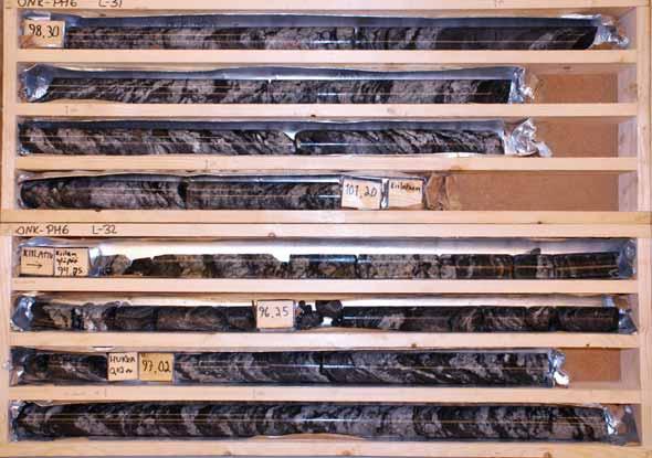
118 109 Appendix 3.10/8

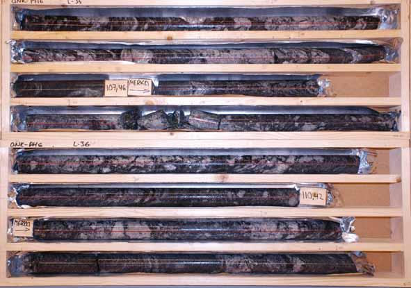
119 110 Appendix 3.10/9

120 111 Appendix 3.10/10

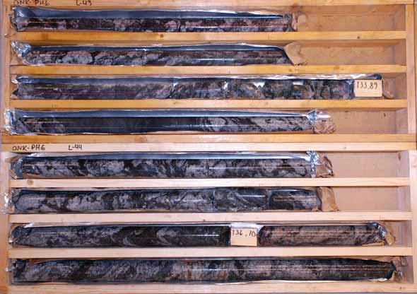
121 112 Appendix 3.10/11

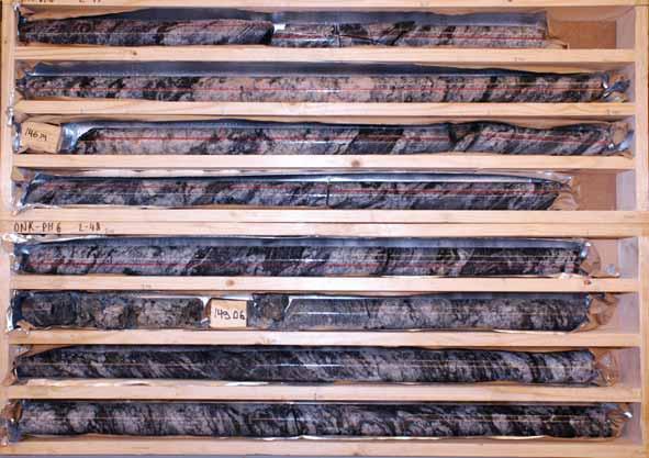
122 113 Appendix 3.10/12

123 114 Appendix 3.10/13

124 115 Appendix 4.1/1 ROCK QUALITY Hole ID: ONK-PH6 Contractor: KATI Oy Northing: Drilling started: Easting: Drilling ended: Elevation: Machine/fixture: ONRAM 1000/4 Direction: 135 Target: PL Dip: -5.7 Purpose: Core diameter: 51 Extension: Casing: 1.4 m Logging date: Remarks: Wedge m, in Geologist: TJUU Max depth: HOLE_ID M_FROM M_TO LENGTH_M > 10 cm Number_of RQD RQD Jn Jr Ja cm fractures % >10 profile median median ONK-PH PRO ONK-PH URO ONK-PH USM ONK-PH URO ONK-PH PRO ONK-PH URO ONK-PH URO ONK-PH URO ONK-PH URO ONK-PH URO ONK-PH URO ONK-PH URO ONK-PH URO ONK-PH URO ONK-PH URO ONK-PH PRO ONK-PH URO ONK-PH PRO ONK-PH URO ONK-PH USM ONK-PH URO ONK-PH URO ONK-PH URO ONK-PH URO ONK-PH URO ONK-PH URO ONK-PH URO ONK-PH URO ONK-PH PRO

125 116 Appendix 4.1/2 HOLE_ID M_FROM M_TO ONK-PH ONK-PH ONK-PH ONK-PH ONK-PH ONK-PH ONK-PH ONK-PH ONK-PH ONK-PH ONK-PH ONK-PH ONK-PH ONK-PH ONK-PH ONK-PH ONK-PH ONK-PH ONK-PH ONK-PH ONK-PH ONK-PH ONK-PH ONK-PH ONK-PH ONK-PH ONK-PH ONK-PH ONK-PH SET 1 SET 2 dip dip dir. Jr Ja Spacing Filling Frac. no. dip dip dir. Jr Ja Spacing Filling Frac. no CC, SK CC, SK, SK SV, CC, KA BT, GR KL, SK, IL, CC SK, SV, CC KA, IL, KL BT,MU,KL,CC,KA KL,SV,SK BT,KA,SK BT,KL,KA KL,KA,SK,IL,SV KA, IL, KL CC,KA,MU CC,KL,IL KA,KL,SV,IL CC,KL,KA IL,KA,CC,SK,KL BT,KL,KA,SK KL,KA,SK KA,SK,KL,BT KA,KL KL,BT,KA,SK CC,KL,KA CC,KA,SV 2

126 117 Appendix 4.1/3 HOLE_ID M_FROM M_TO ONK-PH ONK-PH ONK-PH ONK-PH ONK-PH ONK-PH ONK-PH ONK-PH ONK-PH ONK-PH ONK-PH ONK-PH ONK-PH ONK-PH ONK-PH ONK-PH ONK-PH ONK-PH ONK-PH ONK-PH ONK-PH ONK-PH ONK-PH ONK-PH ONK-PH ONK-PH ONK-PH ONK-PH ONK-PH ROCK_QUALITY_CLASS CLASS_OF_THE Core loss REMARKS GSI GSI Q' FRACTURED_ZONE (m) Q Q STRUCTURE SURF_COND REMARKS Good B 2 77 Exceptionally Good No fractures, Jr B 1 87 No fracture but sparcely fol. Good 29.5 B 2 75 Extremely Good One fracture, Jr B 1 85 Good B 1 85 Very Good No fractures, Jr A 1 85 No fracture but sparcely fol. Very Good A 1 85 Very Good No fractures B 1 85 Very Good B 1 85 Very Good No fractures, Jr B 1 85 Exceptionally Good B 1 85 No fracture but sparcely fol. Very Good B 1 80 Very Good C 1 70 Exceptionally Good No fractures, Jr C 1 75 No fracture but sparcely fol. Very Good A 2 77 Good C 1 70 Exceptionally Good No fractures, Jr C 1 75 No fracture but sparcely fol. Good C 2 63 Very Good B 2 75 Very Good B 1 82 Fair RiII B 2 63 Very Good A 1 77 Exceptionally Good No fractures, Jr A 1 85 No fracture but sparcely fol. Extremely Good B 2 65 Exceptionally Good No fractures, Jr B 1 85 No fracture but sparcely fol. Very Good B 2 60 Exceptionally Good No fractures, Jr B 1 85 No fracture but sparcely fol. Very Good B 2 77 Very Good B 1 85

127 118 Olkiluoto, ONKALO, Borehole ONK-PH6 Flow rate and single point resistance Appendix 5.1 Flow from the measured section (L = 0.5 m, dl = 0.1 m), Interpreted fracture specific flow into the hole Depth (m) Flow rate (ml/h) Single point resistance (ohm)

128 119 Olkiluoto, ONKALO, Borehole ONK-PH6 Flow rate and single point resistance Appendix 5.2 Flow from the measured section (L = 0.5 m, dl = 0.1 m), Interpreted fracture specific flow into the hole Depth (m) Flow rate (ml/h) Single point resistance (ohm)

129 120 Olkiluoto, ONKALO, Borehole ONK-PH6 Flow rate and single point resistance Appendix 5.3 Flow from the measured section (L = 0.5 m, dl = 0.1 m), Interpreted fracture specific flow into the hole Depth (m) Flow rate (ml/h) Single point resistance (ohm)

130 121 Olkiluoto, ONKALO, Borehole ONK-PH6 Flow rate and single point resistance Appendix 5.4 Flow from the measured section (L = 0.5 m, dl = 0.1 m), Interpreted fracture specific flow into the hole Depth (m) Flow rate (ml/h) Single point resistance (ohm)

131 122 Olkiluoto, ONKALO, Borehole ONK-PH6 Flow rate and single point resistance Appendix 5.5 Flow from the measured section (L = 0.5 m, dl = 0.1 m), Interpreted fracture specific flow into the hole Depth (m) Flow rate (ml/h) Single point resistance (ohm)

132 123 Olkiluoto, ONKALO, Borehole ONK-PH6 Flow rate and single point resistance Appendix 5.6 Flow from the measured section (L = 0.5 m, dl = 0.1 m), Interpreted fracture specific flow into the hole Depth (m) Flow rate (ml/h) Single point resistance (ohm)

133 124 Olkiluoto, ONKALO, Borehole ONK-PH6 Flow rate and single point resistance Appendix 5.7 Flow from the measured section (L = 0.5 m, dl = 0.1 m), Interpreted fracture specific flow into the hole Depth (m) Flow rate (ml/h) Single point resistance (ohm)

134 125 Olkiluoto, ONKALO, Borehole ONK-PH6 Flow rate and single point resistance Appendix 5.8 Flow from the measured section (L = 0.5 m, dl = 0.1 m), Interpreted fracture specific flow into the hole Depth (m) Flow rate (ml/h) Single point resistance (ohm)

135 126 Olkiluoto, ONKALO, Borehole ONK-PH6 Plotted transmissivity and hydraulic aperture of detected fractures Appendix 5.9 Hydraulic aperture of fracture (mm) Transmissivity of fracture Depth (m) Hydraulic aperture of fracture (mm) Transmissivity (m 2 /s)

136 127 Appendix 5.10 Hole: PH6 Elevation of the top of the hole (masl): Inclination: Depth of fracture along the borehole (m) Flow (ml/h) Fracture elevation (masl) Drawdown (m) T (m2/s) Hydraulic aperture of fracture (mm) Comments E * E E E * E E E * E E * E E * E E * E E * E E E * E * E E * E E * Uncertain fracture. The flow rate is less than 30 ml/h or the flow anomalies are overlapping or they are unclear because of noise.

137 128 Olkiluoto, ONKALO, Borehole ONK-PH6 Electric conductivity of borehole water Appendix 5.11 During flow logging, upwards (L = 0.5 m, dl = 0.1 m), Depth (m) Electric conductivity (S/m, 25 o C)

138 129 Olkiluoto, ONKALO, Borehole ONK-PH6 Temperature of borehole water Appendix 5.12 During flow logging, upwards (L = 0.5 m, dl = 0.1 m), Depth (m) Temperature ( o C)

139 130 Olkiluoto, ONKALO, Borehole ONK-PH6 Flow rate out from the borehole during flow logging Appendix Flow rate out from the hole (L/min) / 21: / 0: / 3: / 6:00 Year-Month-Day / Hour:Minute / 9: / 12:00

140 131 Appendix 5.14/1 LUGEON TESTS, ONK-PH6 Top Bottom Pressurized Time Pressure Groundwater Effective Water water Amount Lugeon packer packer length used hydrostatic pressure gauge gauge of used value depth depth pressure at start at the end water (m) (m) (m) (min) (bar) (bar) (bar) (litre) 5,04 11,04 6, ,0 14,2 3, , ,0 7,1 0,31 5,04 11,04 6, ,0 14,2 7, , ,2 3,2 0,07 5,04 11,04 6, ,0 14,2 10, , ,9 2,0 0,03 5,04 11,04 6, ,0 14,2 7, , ,6 1,7 0,04 5,04 11,04 6, ,0 14,2 3, , ,8 0,2 0,01 11,04 17,04 6, ,0 14,3 3, , ,9 2,1 0,09 11,04 17,04 6, ,0 14,3 7, , ,9 2,3 0,05 11,04 17,04 6, ,0 14,3 10, , ,9 2,5 0,04 11,04 17,04 6, ,0 14,3 7, , ,2 1,3 0,03 11,04 17,04 6, ,0 14,3 3, , ,8 0,6 0,03 17,04 23,04 6, ,0 14,3 3, , ,2 0,3 0,01 17,04 23,04 6, ,0 14,3 7, , ,3 0,1 0,00 17,04 23,04 6, ,0 14,3 10, , ,5 0,1 0,00 17,04 23,04 6, ,0 14,3 7, , ,7 0,2 0,00 17,04 23,04 6, ,0 14,3 3, , ,7 0,0 0,00 23,04 29,04 6, ,0 14,4 3, , ,3 0,0 0,00 23,04 29,04 6, ,0 14,4 7, , ,3 0,1 0,00 23,04 29,04 6, ,0 14,4 10, , ,5 0,3 0,00 23,04 29,04 6, ,0 14,4 7, , ,6 0,1 0,00 23,04 29,04 6, ,0 14,4 3, , ,6 0,0 0,00 29,04 35,04 6, ,0 14,5 3, , ,2 4,6 0,22 29,04 35,04 6, ,0 14,5 7, , ,1 3,3 0,07 29,04 35,04 6, ,0 14,5 10, , ,5 2,9 0,05 29,04 35,04 6, ,0 14,5 7, , ,2 1,7 0,04 29,04 35,04 6, ,0 14,5 3, , ,7 0,5 0,02 35,04 41,04 6, ,0 14,5 3, , ,4 0,0 0,00 35,04 41,04 6, ,0 14,5 7, , ,2 0,0 0,00 35,04 41,04 6, ,0 14,5 10, , ,2 0,0 0,00 35,04 41,04 6, ,0 14,5 7, , ,2 0,0 0,00 35,04 41,04 6, ,0 14,5 3, , ,2 0,0 0,00 41,04 47,04 6, ,0 14,6 3, , ,5 1,4 0,07 41,04 47,04 6, ,0 14,6 7, , ,2 0,0 0,00 41,04 47,04 6, ,0 14,6 10, , ,6 0,8 0,01 41,04 47,04 6, ,0 14,6 7, , ,2 0,6 0,01 41,04 47,04 6, ,0 14,6 3, , ,2 0,0 0,00 47,04 53,04 6, ,0 14,6 3, , ,3 0,0 0,00 47,04 53,04 6, ,0 14,6 7, , ,3 0,0 0,00 47,04 53,04 6, ,0 14,6 10, , ,9 0,9 0,01 47,04 53,04 6, ,0 14,6 7, , ,9 0,0 0,00 47,04 53,04 6, ,0 14,6 3, , ,9 0,0 0,00 53,04 59,04 6, ,0 14,7 3, , ,9 0,4 0,02 53,04 59,04 6, ,0 14,7 7, , ,5 0,6 0,01 53,04 59,04 6, ,0 14,7 10, , ,5 0,4 0,01 53,04 59,04 6, ,0 14,7 7, , ,5 0,0 0,00 53,04 59,04 6, ,0 14,7 3, , ,5 0,0 0,00 59,04 65,04 6, ,0 14,7 3, , ,2 0,0 0,00

141 132 Appendix 5.14/2 59,04 65,04 6, ,0 14,7 7, , ,3 0,2 0,00 59,04 65,04 6, ,0 14,7 10, , ,2 0,1 0,00 59,04 65,04 6, ,0 14,7 7, , ,2 0,0 0,00 59,04 65,04 6, ,0 14,7 3, , ,2 0,0 0,00 65,04 71,04 6, ,0 14,8 3, , ,2 0,7 0,04 65,04 71,04 6, ,0 14,8 7, , ,9 1,1 0,03 65,04 71,04 6, ,0 14,8 10, , ,1 0,6 0,01 65,04 71,04 6, ,0 14,8 7, , ,5 0,4 0,01 65,04 71,04 6, ,0 14,8 3, , ,5 0,0 0,00 71,04 77,04 6, ,0 14,9 3, , ,5 0,0 0,00 71,04 77,04 6, ,0 14,9 7, , ,5 1,1 0,03 71,04 77,04 6, ,0 14,9 10, , ,9 4,5 0,07 71,04 77,04 6, ,0 14,9 7, , ,9 0,0 0,00 71,04 77,04 6, ,0 14,9 3, , ,9 0,0 0,00 77,04 83,04 6, ,0 14,9 3, , ,1 6,6 0,36 77,04 83,04 6, ,0 14,9 7, , ,1 8,4 0,20 77,04 83,04 6, ,0 14,9 10, , ,6 8,5 0,14 77,04 83,04 6, ,0 14,9 7, , ,1 9,3 0,22 77,04 83,04 6, ,0 14,9 3, , ,3 6,2 0,34 83,04 89,04 6, ,0 15,0 3, , ,8 7,8 0,43 83,04 89,04 6, ,0 15,0 7, , ,0 9,7 0,23 83,04 89,04 6, ,0 15,0 10, , ,3 11,1 0,18 83,04 89,04 6, ,0 15,0 7, , ,1 8,9 0,21 83,04 89,04 6, ,0 15,0 3, , ,2 6,1 0,34 89,04 95,04 6, ,0 15,0 3,0 0,0 0,0 0,0 0,00 89,04 95,04 6, ,0 15,0 7,0 0,0 0,0 0,0 0,00 89,04 95,04 6, ,0 15,0 10,0 0,0 0,0 0,0 0,00 89,04 95,04 6, ,0 15,0 7,0 0,0 0,0 0,0 0,00 89,04 95,04 6, ,0 15,0 3,0 0,0 0,0 0,0 0,00 95,04 101,04 6, ,0 15,1 2,9 0,0 0,0 0,0 0,00 95,04 101,04 6, ,0 15,1 6,9 0,0 0,0 0,0 0,00 95,04 101,04 6, ,0 15,1 9,9 0,0 0,0 0,0 0,00 95,04 101,04 6, ,0 15,1 6,9 0,0 0,0 0,0 0,00 95,04 101,04 6, ,0 15,1 2,9 0,0 0,0 0,0 0,00 101,04 107,04 6, ,0 15,2 2, , ,9 23,3 1,36 101,04 107,04 6, ,0 15,2 6, , ,3 26,5 0,65 101,04 107,04 6, ,0 15,2 9, , ,9 28,5 0,48 101,04 107,04 6, ,0 15,2 6, , ,2 26,3 0,64 101,04 107,04 6, ,0 15,2 2, , ,6 19,4 1,14 107,04 113,04 6, ,0 15,2 2, , ,9 14,1 0,84 107,04 113,04 6, ,0 15,2 6, , ,6 13,5 0,33 107,04 113,04 6, ,0 15,2 9, , ,8 15,1 0,26 107,04 113,04 6, ,0 15,2 6, , ,1 11,3 0,28 107,04 113,04 6, ,0 15,2 2, , ,5 9,4 0,56 113,04 119,04 6, ,0 15,3 2, , ,4 2,5 0,15 113,04 119,04 6, ,0 15,3 6, , ,2 2,6 0,06 113,04 119,04 6, ,0 15,3 9, , ,2 2,5 0,04 113,04 119,04 6, ,0 15,3 6, , ,7 1,5 0,04 113,04 119,04 6, ,0 15,3 2, , ,8 1,1 0,07 119,04 125,04 6, ,0 15,3 2, , ,9 6,8 0,42 119,04 125,04 6, ,0 15,3 6, , ,9 11,0 0,27 119,04 125,04 6, ,0 15,3 9, , ,1 11,2 0,19

142 133 Appendix 5.14/3 119,04 125,04 6, ,0 15,3 6, , ,5 6,4 0,16 119,04 125,04 6, ,0 15,3 2, , ,4 3,9 0,24 125,04 131,04 6, ,0 15,4 2, , ,8 4,6 0,29 125,04 131,04 6, ,0 15,4 6, , ,9 10,1 0,25 125,04 131,04 6, ,0 15,4 9, , ,8 8,9 0,15 125,04 131,04 6, ,0 15,4 6, , ,9 7,1 0,18 125,04 131,04 6, ,0 15,4 2, , ,2 3,3 0,21 131,04 137,04 6, ,0 15,4 2, , ,1 11,2 0,73 131,04 137,04 6, ,0 15,4 6, , ,1 12,0 0,31 131,04 137,04 6, ,0 15,4 9, , ,0 11,9 0,21 131,04 137,04 6, ,0 15,4 6, , ,6 13,6 0,35 131,04 137,04 6, ,0 15,4 2, , ,3 11,7 0,76 137,04 143,04 6, ,0 15,5 2, , ,6 11,5 0,77 137,04 143,04 6, ,0 15,5 6, , ,8 19,2 0,49 137,04 143,04 6, ,0 15,5 9, , ,3 17,5 0,31 137,04 143,04 6, ,0 15,5 6, , ,9 12,6 0,32 137,04 143,04 6, ,0 15,5 2, , ,5 8,6 0,57 143,04 149,04 6, ,0 15,6 2, , ,2 13,1 0,89 143,04 149,04 6, ,0 15,6 6, , ,2 14,0 0,36 143,04 149,04 6, ,0 15,6 9, , ,7 16,5 0,29 143,04 149,04 6, ,0 15,6 6, , ,1 9,4 0,24 143,04 149,04 6, ,0 15,6 2, , ,3 9,2 0,63 149,04 155,04 6, ,0 15,6 2, , ,0 12,9 0,90 149,04 155,04 6, ,0 15,6 6, , ,6 15,6 0,41 149,04 155,04 6, ,0 15,6 9, , ,4 22,8 0,40 149,04 155,04 6, ,0 15,6 6, , ,2 16,8 0,44 149,04 155,04 6, ,0 15,6 2, , ,2 14,0 0,98 air pressure 1,01324 gravitation 0,0981 sin 5,6425 0,10 collar elevation -128,21 groundwater table 6

143 134 Appendix 5.15/1 LUGEON TESTS, ONK-PH6, INTERPRETED VALUES (Inclination: -5,6425 degrees) Sorting Depth of Depth of Length of Time Used Hydrostatic Used Reading ofreading of water Lugeon Interpreted index lower end of upper end of measuring pressure pressure of (actual) water water loss value Lugeon upper packer lower packer section groundwater pressure gauge, gauge, value (m) (m) (m) (min) (bar) (bar) (bar) start end (litre) 5,04 5,04 11,04 6, ,0 14,2 3, , ,0 7,1 0,31 5,54 5,04 11,04 6, ,0 14,2 7, , ,2 3,2 0,07 6,04 5,04 11,04 6, ,0 14,2 10, , ,9 2,0 0,03 0,01 6,54 5,04 11,04 6, ,0 14,2 7, , ,6 1,7 0,04 7,04 5,04 11,04 6, ,0 14,2 3, , ,8 0,2 0,01 7,54 11,04 11,04 17,04 6, ,0 14,3 3, , ,9 2,1 0,09 11,54 11,04 17,04 6, ,0 14,3 7, , ,9 2,3 0,05 12,04 11,04 17,04 6, ,0 14,3 10, , ,9 2,5 0,04 0,03 12,54 11,04 17,04 6, ,0 14,3 7, , ,2 1,3 0,03 13,04 11,04 17,04 6, ,0 14,3 3, , ,8 0,6 0,03 13,54 17,04 17,04 23,04 6, ,0 14,3 3, , ,2 0,3 0,01 17,54 17,04 23,04 6, ,0 14,3 7, , ,3 0,1 0,00 18,04 17,04 23,04 6, ,0 14,3 10, , ,5 0,1 0,00 0,00 18,54 17,04 23,04 6, ,0 14,3 7, , ,7 0,2 0,00 19,04 17,04 23,04 6, ,0 14,3 3, , ,7 0,0 0,00 19,54 23,04 23,04 29,04 6, ,0 14,4 3, , ,3 0,0 0,00 23,54 23,04 29,04 6, ,0 14,4 7, , ,3 0,1 0,00 24,04 23,04 29,04 6, ,0 14,4 10, , ,5 0,3 0,00 0,00 24,54 23,04 29,04 6, ,0 14,4 7, , ,6 0,1 0,00 25,04 23,04 29,04 6, ,0 14,4 3, , ,6 0,0 0,00 25,54 29,04 29,04 35,04 6, ,0 14,5 3, , ,2 4,6 0,22 29,54 29,04 35,04 6, ,0 14,5 7, , ,1 3,3 0,07 30,04 29,04 35,04 6, ,0 14,5 10, , ,5 2,9 0,05 0,04 30,54 29,04 35,04 6, ,0 14,5 7, , ,2 1,7 0,04 31,04 29,04 35,04 6, ,0 14,5 3, , ,7 0,5 0,02 31,54 35,04 35,04 41,04 6, ,0 14,5 3, , ,4 0,0 0,00 35,54 35,04 41,04 6, ,0 14,5 7, , ,2 0,0 0,00 36,04 35,04 41,04 6, ,0 14,5 10, , ,2 0,0 0,00 0,00 36,54 35,04 41,04 6, ,0 14,5 7, , ,2 0,0 0,00 37,04 35,04 41,04 6, ,0 14,5 3, , ,2 0,0 0,00 37,54 41,04 41,04 47,04 6, ,0 14,6 3, , ,5 1,4 0,07 41,54 41,04 47,04 6, ,0 14,6 7, , ,2 0,0 0,00 42,04 41,04 47,04 6, ,0 14,6 10, , ,6 0,8 0,01 0,00 42,54 41,04 47,04 6, ,0 14,6 7, , ,2 0,6 0,01 43,04 41,04 47,04 6, ,0 14,6 3, , ,2 0,0 0,00 43,54 47,04 47,04 53,04 6, ,0 14,6 3, , ,3 0,0 0,00 47,54 47,04 53,04 6, ,0 14,6 7, , ,3 0,0 0,00 48,04 47,04 53,04 6, ,0 14,6 10, , ,9 0,9 0,01 0,00 48,54 47,04 53,04 6, ,0 14,6 7, , ,9 0,0 0,00 49,04 47,04 53,04 6, ,0 14,6 3, , ,9 0,0 0,00 49,54 53,04 53,04 59,04 6, ,0 14,7 3, , ,9 0,4 0,02 53,54 53,04 59,04 6, ,0 14,7 7, , ,5 0,6 0,01 54,04 53,04 59,04 6, ,0 14,7 10, , ,5 0,4 0,01 0,00 54,54 53,04 59,04 6, ,0 14,7 7, , ,5 0,0 0,00 55,04 53,04 59,04 6, ,0 14,7 3, , ,5 0,0 0,00 55,54 59,04 59,04 65,04 6, ,0 14,7 3, , ,2 0,0 0,00 59,54 59,04 65,04 6, ,0 14,7 7, , ,3 0,2 0,00 60,04 59,04 65,04 6, ,0 14,7 10, , ,2 0,1 0,00 0,00 60,54 59,04 65,04 6, ,0 14,7 7, , ,2 0,0 0,00 61,04 59,04 65,04 6, ,0 14,7 3, , ,2 0,0 0,00 61,54 65,04 65,04 71,04 6, ,0 14,8 3, , ,2 0,7 0,04 65,54 65,04 71,04 6, ,0 14,8 7, , ,9 1,1 0,03 66,04 65,04 71,04 6, ,0 14,8 10, , ,1 0,6 0,01 0,00 66,54 65,04 71,04 6, ,0 14,8 7, , ,5 0,4 0,01 67,04 65,04 71,04 6, ,0 14,8 3, , ,5 0,0 0,00 67,54 71,04 71,04 77,04 6, ,0 14,9 3, , ,5 0,0 0,00 71,54 71,04 77,04 6, ,0 14,9 7, , ,5 1,1 0,03 72,04 71,04 77,04 6, ,0 14,9 10, , ,9 4,5 0,07 0,00 72,54 71,04 77,04 6, ,0 14,9 7, , ,9 0,0 0,00 73,04 71,04 77,04 6, ,0 14,9 3, , ,9 0,0 0,00 73,54 77,04 77,04 83,04 6, ,0 14,9 3, , ,1 6,6 0,36 77,54 77,04 83,04 6, ,0 14,9 7, , ,1 8,4 0,20 78,04 77,04 83,04 6, ,0 14,9 10, , ,6 8,5 0,14 0,14 78,54 77,04 83,04 6, ,0 14,9 7, , ,1 9,3 0,22 79,04 77,04 83,04 6, ,0 14,9 3, , ,3 6,2 0,34 79,54 83,04 83,04 89,04 6, ,0 15,0 3, , ,8 7,8 0,43

144 135 Appendix 5.15/2 83,54 83,04 89,04 6, ,0 15,0 7, , ,0 9,7 0,23 84,04 83,04 89,04 6, ,0 15,0 10, , ,3 11,1 0,18 0,18 84,54 83,04 89,04 6, ,0 15,0 7, , ,1 8,9 0,21 85,04 83,04 89,04 6, ,0 15,0 3, , ,2 6,1 0,34 85,54 89,04 89,04 95,04 6, ,0 15,0 3,0 0,0 0,0 0,0 0,00 wedge, no measurements 89,54 89,04 95,04 6, ,0 15,0 7,0 0,0 0,0 0,0 0,00 wedge, no measurements 90,04 89,04 95,04 6, ,0 15,0 10,0 0,0 0,0 0,0 0,00 wedge, no measurements 90,54 89,04 95,04 6, ,0 15,0 7,0 0,0 0,0 0,0 0,00 wedge, no measurements 91,04 89,04 95,04 6, ,0 15,0 3,0 0,0 0,0 0,0 0,00 wedge, no measurements 91,54 95,04 95,04 101,04 6, ,0 15,1 2,9 0,0 0,0 0,0 0,00 wedge, no measurements 95,54 95,04 101,04 6, ,0 15,1 6,9 0,0 0,0 0,0 0,00 wedge, no measurements 96,04 95,04 101,04 6, ,0 15,1 9,9 0,0 0,0 0,0 0,00 wedge, no measurements 96,54 95,04 101,04 6, ,0 15,1 6,9 0,0 0,0 0,0 0,00 wedge, no measurements 97,04 95,04 101,04 6, ,0 15,1 2,9 0,0 0,0 0,0 0,00 wedge, no measurements 97,54 101,04 101,04 107,04 6, ,0 15,2 2, , ,9 23,3 1,36 101,54 101,04 107,04 6, ,0 15,2 6, , ,3 26,5 0,65 102,04 101,04 107,04 6, ,0 15,2 9, , ,9 28,5 0,48 0,48 102,54 101,04 107,04 6, ,0 15,2 6, , ,2 26,3 0,64 103,04 101,04 107,04 6, ,0 15,2 2, , ,6 19,4 1,14 103,54 107,04 107,04 113,04 6, ,0 15,2 2, , ,9 14,1 0,84 107,54 107,04 113,04 6, ,0 15,2 6, , ,6 13,5 0,33 108,04 107,04 113,04 6, ,0 15,2 9, , ,8 15,1 0,26 0,26 108,54 107,04 113,04 6, ,0 15,2 6, , ,1 11,3 0,28 109,04 107,04 113,04 6, ,0 15,2 2, , ,5 9,4 0,56 109,54 113,04 113,04 119,04 6, ,0 15,3 2, , ,4 2,5 0,15 113,54 113,04 119,04 6, ,0 15,3 6, , ,2 2,6 0,06 114,04 113,04 119,04 6, ,0 15,3 9, , ,2 2,5 0,04 0,04 114,54 113,04 119,04 6, ,0 15,3 6, , ,7 1,5 0,04 115,04 113,04 119,04 6, ,0 15,3 2, , ,8 1,1 0,07 115,54 119,04 119,04 125,04 6, ,0 15,3 2, , ,9 6,8 0,42 119,54 119,04 125,04 6, ,0 15,3 6, , ,9 11,0 0,27 120,04 119,04 125,04 6, ,0 15,3 9, , ,1 11,2 0,19 0,19 120,54 119,04 125,04 6, ,0 15,3 6, , ,5 6,4 0,16 121,04 119,04 125,04 6, ,0 15,3 2, , ,4 3,9 0,24 121,54 125,04 125,04 131,04 6, ,0 15,4 2, , ,8 4,6 0,29 125,54 125,04 131,04 6, ,0 15,4 6, , ,9 10,1 0,25 126,04 125,04 131,04 6, ,0 15,4 9, , ,8 8,9 0,15 0,15 126,54 125,04 131,04 6, ,0 15,4 6, , ,9 7,1 0,18 127,04 125,04 131,04 6, ,0 15,4 2, , ,2 3,3 0,21 127,54 131,04 131,04 137,04 6, ,0 15,4 2, , ,1 11,2 0,73 131,54 131,04 137,04 6, ,0 15,4 6, , ,1 12,0 0,31 132,04 131,04 137,04 6, ,0 15,4 9, , ,0 11,9 0,21 0,21 132,54 131,04 137,04 6, ,0 15,4 6, , ,6 13,6 0,35 133,04 131,04 137,04 6, ,0 15,4 2, , ,3 11,7 0,76 133,54 137,04 137,04 143,04 6, ,0 15,5 2, , ,6 11,5 0,77 137,54 137,04 143,04 6, ,0 15,5 6, , ,8 19,2 0,49 138,04 137,04 143,04 6, ,0 15,5 9, , ,3 17,5 0,31 0,31 138,54 137,04 143,04 6, ,0 15,5 6, , ,9 12,6 0,32 139,04 137,04 143,04 6, ,0 15,5 2, , ,5 8,6 0,57 139,54 143,04 143,04 149,04 6, ,0 15,6 2, , ,2 13,1 0,89 143,54 143,04 149,04 6, ,0 15,6 6, , ,2 14,0 0,36 144,04 143,04 149,04 6, ,0 15,6 9, , ,7 16,5 0,29 0,29 144,54 143,04 149,04 6, ,0 15,6 6, , ,1 9,4 0,24 145,04 143,04 149,04 6, ,0 15,6 2, , ,3 9,2 0,63 145,54 149,04 149,04 155,04 6, ,0 15,6 2, , ,0 12,9 0,90 149,54 149,04 155,04 6, ,0 15,6 6, , ,6 15,6 0,41 150,04 149,04 155,04 6, ,0 15,6 9, , ,4 22,8 0,40 0,40 150,54 149,04 155,04 6, ,0 15,6 6, , ,2 16,8 0,44 151,04 149,04 155,04 6, ,0 15,6 2, , ,2 14,0 0,98 151,54 air pressure 1,01324 press. of water column 0,0981 sin 0,10 collar -128,21 groundwater table 6,00 water column 134,205

145 136 Appendix 6.1/1 Borehole Logging Suomen Malmi Oy P.O. Box 10 FI ESPOO Client: Posiva Oy Hole no: ONK-PH06 Ø: 76 Surveyed by:vs, AS Site: Olkiluoto X: Length: Survey date: Project no: 9868/06/TUAH Y: Azimuth: 135 Reported by: AT Z: Dip: -5.7 Report date: Lith. Fracture Freq. Depth Chainage Gamma-Gamma Density Short Normal Resistivity N16" Radar Arrival Time P Velocity 0.6 m 0 1/m g/cm Ohm.m nanosec m/s 6500 Core loss 1m:500m Natural Gamma Radiation 0 MicroR/h 150 Long Normal Resistivity N64" 2 Ohm.m Radar apparent velocity 50 m/microsec 150 S Velocity 0.6 m 2000 m/s 4000 Ri Susceptibility Resistance Single Point Radar amplitude 0 1E Ohm microvolt Wenner 30cm 2 Ohm.m

146 137 Appendix 6.1/

147 138 Appendix 6.2/1 Borehole Radar Suomen Malmi Oy P.O. Box 10 FI ESPOO Client: Posiva Oy Hole no: ONK-PH06 Ø: 76 Surveyed by:vs, AS Site: Olkiluoto X: Length: Survey date: Project no: 9868/06/TUAH Y: Azimuth: 135 Reported by: AT Z: Dip: -5.7 Report date: Lith. Fracture Freq. Depth Chainage Radar Arrival Time Radar Raw Image 250 MHz 0 1/m 10 Core loss Ri 1m:500m 40 nanosec 18 Radar apparent velocity 50 m/microsec 150 Radar amplitude Velocity 117 m/microsec (.25 microsec = c. 15 m) microvolt

148 139 Appendix 6.2/

149 140 Appendix 6.3/1 Suomen Malmi Oy P.O. Box 10 FI ESPOO Borehole Radar Client: Posiva Oy Hole no: ONK-PH06 Ø: 76 Surveyed by:vs, AS Site: Olkiluoto X: Length: Survey date: Project no: 9868/06/TUAH Y: Azimuth: 135 Reported by: AT Z: Dip: -5.7 Report date: Lith. Fracture Freq. Depth Chainage Fracture Intersection Fracture Orientation Radar Orientations Refl.Ext Backwd 0 1/m 10 1m:200m Schmidt Plot - Lower Hemisphere 30 m 0 Core Foliation Intersection Foliation Orientation loss Ri Radar Intersection Radar Orientation Schmidt Plot - Lower Hemisphere Depth: 0.00 [m] to [m] Mean Counts 8 Dip[deg] Azi[deg] Refl.Ext Forwd 0 m 30 Range Out 0 m 15

150 141 Appendix 6.3/ Schmidt Plot - Lower Hemisphere Depth: [m] to [m] Mean Counts 8 Dip[deg] Azi[deg] Schmidt Plot - Lower Hemisphere Depth: [m] to [m] Mean Counts 16 Dip[deg] Azi[deg]

151 142 Appendix 6.3/ Schmidt Plot - Lower Hemisphere Depth: [m] to [m] Mean Counts 16 Dip[deg] Azi[deg] Schmidt Plot - Lower Hemisphere Depth: [m] to [m] Mean Counts 15 Dip[deg] Azi[deg]

152 143 Appendix 6.3/ Schmidt Plot - Lower Hemisphere Depth: [m] to [m] Mean Counts 13 Dip[deg] Azi[deg] Schmidt Plot - Lower Hemisphere Depth: [m] to [m] Mean Counts 13 Dip[deg] Azi[deg]

153 144 Appendix 6.3/ Schmidt Plot - Lower Hemisphere Depth: [m] to [m] Mean Counts 7 Dip[deg] Azi[deg] Schmidt Plot - Lower Hemisphere Depth: [m] to [m] 0

154 145 Appendix 6.3/ Mean 180 Counts 25 Dip[deg] Azi[deg]

155 146 Appendix 6.4/1 Angle, deg Azimuth, deg Dip,deg Ext. Back,m ward Ext. Forward, m Range out, m CLASS Comment FILTER TYPE Nr. Depth,m PLANE not orient before borehole no filter PLANE L not orient no filter PLANE L not orient no filter PLANE L not orient no filter FractureOrient, weak, before borehole no filt PLANE L PLANE L not orient NF PLANE L not orient NF PLANE L FractureOrient NF FoliationOrient or tunnel wall No filt. PLANE L PLANE L FoliationOrient NF PLANE L not orient NF PLANE L FoliationOrient NF PLANE L FoliationOrient NF PLANE L FractureOrient NF PLANE L FractureOrient FIR PLANE L not orient PLANE L FoliationOrient HFIR PLANE L not orient NF FoliationOrient. Conductive, delay. HFIR PLANE L PLANE L not orient NF PLANE L not orient NF PLANE L FractureOrient(Fol) NF PLANE L FractureOrient HFIR PLANE L FoliationOrient FIR PLANE L FractureOrient NF PLANE L not orient NF PLANE L FractureOrient NF PLANE L not orient

156 147 Appendix 6.4/2 PLANE L FractureOrient PLANE L FractureOrient HFIR PLANE L not orient PLANE L not orient NF PLANE L FractureOrient PLANE L not orient PLANE L FractureOrient(Clay) PLANE L FractureOrient PLANE L FractureOrient PLANE L FoliationOrient NF FractureOrient, Conductive, Delay PLANE L PLANE L FoliationOrient HFIR PLANE L FoliationOrient HFIR PLANE L FoliationOrient NF PLANE L not orient NF PLANE L FoliationOrient NF PLANE L FractureOrient PLANE L not orient PLANE L FractureOrient PLANE L not orient NF PLANE L FoliationOrient PLANE L not orient NF PLANE L not orient HFIR PLANE L FoliationOrient NF PLANE L FoliationOrient PLANE L FractureOrient NF PLANE L FoliationOrient PLANE L FractureOrientation PLANE L not orient Strong, close PLANE L FoliationOrient FIR PLANE L FoliationOrient NF

157 148 Appendix 6.4/3 PLANE L FoliationOrient NF FractureOrient, PLANE L Conductive, Delay NF PLANE L FractureOrient NF PLANE L not orient NF PLANE L not orient HFIR PLANE L FoliationOrient HFIR PLANE L not orient Stong, far NF PLANE L FoliationOrient FIR PLANE L FractureOrient PLANE L FractureOrient? PLANE L FoliationOrient PLANE L PLANE L FractureOrient PLANE L FoliationOrient PLANE L FoliationOrient, Conductive, Delay HFIR FractureOrient, Conductive, Delay FoliationOrient, Conductive, Delay PLANE L FoliationOrient, PLANE L Conductive, Delay NF PLANE L FoliationOrient NF PLANE L FractureOrient PLANE L FoliationOrient NF PLANE L not orient NF PLANE L FoliationOrient PLANE L FractureOrient NF PLANE L not orient PLANE L FoliationOrient NF FoliationOrient, Conductive, Delay NF PLANE L PLANE L not orient HFIR

158 149 Appendix 6.4/4 PLANE L FractureOrient PLANE L not orient PLANE L FoliationOrient PLANE L FoliationOrient NF PLANE L FoliationOrient PLANE L FractureOrient PLANE L FoliationOrient PLANE L not orient PLANE L FractureOrient FoliationOrient, Conductive, Delay PLANE L PLANE L FoliationOrient PLANE L not orient HFIR PLANE L FoliationOrient(30deg) PLANE L FoliationOrient NF PLANE L FractureOrient NF PLANE L FractureOrient FoliationOrient, Conductive, Delay HFIR PLANE L PLANE L not orient PLANE L FractureOrient PLANE L not orient PLANE L not orient PLANE L FoliationOrient PLANE L FractureOrient PLANE L FractureOrient FIR PLANE L not orient PLANE L FractureOrient PLANE L not orient PLANE L FractureOrient FIR PLANE L FractureOrient PLANE L not orient Wedge? PLANE L FoliationOrient

159 150 Appendix 6.4/5 PLANE L FractureOrient HFIR PLANE L not orient PLANE L FoliationOrient(Fract) PLANE L FractureOrient FIR PLANE L not orient FoliationOrient(25deg), Conductive, Delay PLANE L PLANE L not orient NF PLANE L FoliationOrient PLANE L not orient PLANE L FractureOrient PLANE L FoliationOrient Hfir PLANE L FoliationOrient PLANE L FoliationOrient PLANE L not orient FIR PLANE L FoliationOrient PLANE L not orient PLANE L not orient PLANE L FoliationOrient(25deg) PLANE L FoliationOrient(35deg) PLANE L FoliationOrient PLANE L FoliationOrient hfir PLANE L not orient Conductive, Delay FoliationOrient(25deg), Conductive, Delay HFIR PLANE L PLANE L not orient Conductive, Delay PLANE L PLANE L FractureOrient, Conductive, Delay FoliationOrient, Conductive, Delay FoliationOrient, Conductive, Delay PLANE L PLANE L FractureOrient,

160 151 Appendix 6.4/6 PLANE L PLANE L PLANE L PLANE L Conductive, Delay FractureOrient, Conductive, Delay FoliationOrient, Conductive, Delay FoliationOrient, Conductive, Delay FoliationOrient, Conductive, Delay FractureOrient, Conductive, Delay PLANE L PLANE L not orient Conductive, Delay PLANE L FoliationOrient, Conductive, Delay FoliationOrient, Conductive, Delay PLANE L FractureOrient, PLANE L Conductive, Delay FIR PLANE L FoliationOrient HFIR PLANE L FoliationOrient PLANE L not orient Conductive, Delay PLANE L not orient Conductive, Delay PLANE L FractureOrient HFIR PLANE L FractureOrient HFIR PLANE L not orient PLANE L FractureOrient PLANE L not orient PLANE L FoliationOrient PLANE L FractureOrient PLANE L FractureOrient PLANE L FoliationOrient HFIR PLANE L FractureOrient HFIR PLANE L not orient PLANE L FoliationOrient

161 152 Appendix 6.4/7 PLANE L FoliationOrient PLANE L FoliationOrient PLANE L not orient HFIR PLANE L FoliationOrient PLANE L not orient PLANE L not orient PLANE L not orient PLANE L not orient PLANE L not orient PLANE L not orient Type Distance NR Depth POINT P POINT P POINT P POINT P POINT P POINT P POINT P POINT P POINT P

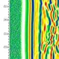
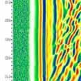
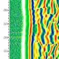
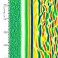
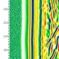
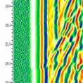
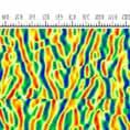
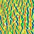
162 153 Appendix 6.5/1

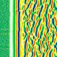
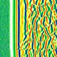
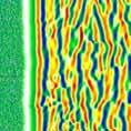
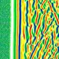
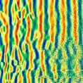
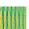
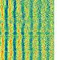
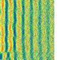
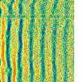
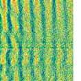
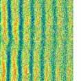
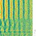
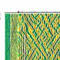
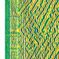
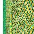
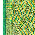
163 154 Appendix 6.5/2

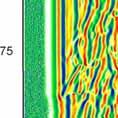
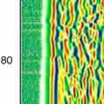
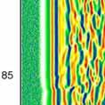
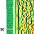
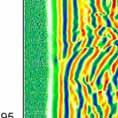
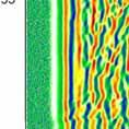
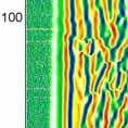
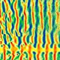
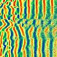
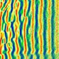
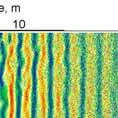
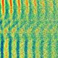
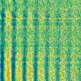
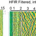
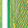
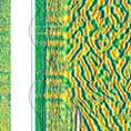
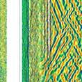
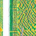
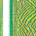
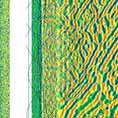
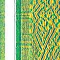
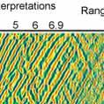
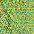
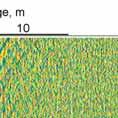
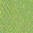
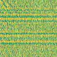
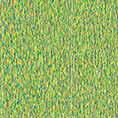
164 155 Appendix 6.5/3

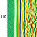
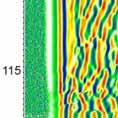
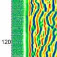
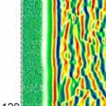
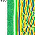
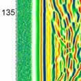
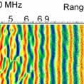
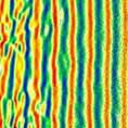
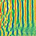
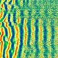
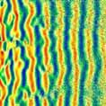
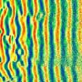
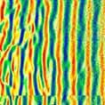
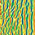
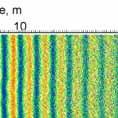
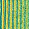
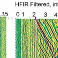
165 156 Appendix 6.5/4

166 157 Appendix 6.6/1 Acoustic Logging Suomen Malmi Oy P.O. Box 10 FI ESPOO Client: Posiva Oy Hole no: ONK-PH06 Ø: 76 Surveyed by:vs, AS Site: Olkiluoto X: Length: Survey date: Project no: 9868/06/TUAH Y: Azimuth: 135 Reported by: AT Z: Dip: -5.7 Report date: Lith. Fracture Freq. Depth Chainage P Velocity 0.6 m Full Wave Sonic, 0.6 m Full Wave Sonic, 1 m 0 1/m 10 Ri 1m:500m 4000 m/s 6500 S Velocity 0.6 m -50 microsec microsec m/s 4000 Core loss

167 158 Appendix 6.6/

168 159 Appendix 6.7/1 Acoustic Logging Suomen Malmi Oy P.O. Box 10 FI ESPOO Client: Posiva Oy Hole no: ONK-PH06 Ø: 76 Surveyed by:vs, AS Site: Olkiluoto X: Length: Survey date: Project no: 9868/06/TUAH Y: Azimuth: 135 Reported by: AT Z: Dip: -5.7 Report date: Lith. Fracture Freq. Depth Chainage P Velocity 0.6 m Gamma-gamma Density Poisson's Ratio P Attenuation Tubewave En. RX1 0 1/m 10 Ri Core 1m:500m 4000 m/s 6500 P Velocity 1 m 4000 m/s 6500 S Velocity 0.6 m 2.5 g/cm3 3.2 Apparent Q (Barton 2002) Shear Modulus 10 GPa 50 Young's Modulus -60 db/m 60 S Attenuation -60 db/m Tubewave En. RX Tubewave Attenuation loss 2000 m/s GPa db/m 70 S Velocity 1 m Bulk Modulus 2000 m/s GPa 200 Bulk Comp 0 1/MPa

169 160 Appendix 6.7/

170 161 Optical Imaging Suomen Malmi Oy P.O. Box 10 FI ESPOO Appendix 6.8 Client: Posiva Oy Hole no: ONK-PH06 Ø: 76 Surveyed by:vs, AS Site: Olkiluoto X: Length: Survey date: Project no:9868/06/tuah Y: Azimuth: 135 Reported by: AT Z: Dip: -5.7 Report date: Depth ONK-PH06 3D Log Elevation Chainage PH06 Image m 1m:4m 0 Depth Corrected. Oriented to High Side (180=Bottom)

171 162 Appendix 6.9/1

172 163 Appendix 6.9/2

173 164 Appendix 6.10 Rautaruukki RROM-2 Specifications Antenna dimensions -diameter 42 mm -length 1570 mm -electrode separation a=318 mm -diameter of the electrodes 40 mm Measuring cable minimum 4-conductor, length up to 1000 m, loop resistance for output voltage conductors max 40 Ohm Measuring current 10 ma/20 Hz Range Ohm-m Output voltage +5 V -6 V Power feed 18 V, 3 Ah Power consumption 2.4 W Operation temperature C U 4 a I 1 a m 0.318m = resistivity U = voltage I = current

174 Logging Sondes 165 Appendix 6.11 Normal Resistivity Sonde The Geovista digital Normal Resistivity Sonde can be used on its own or in combination with other Geovista sondes for efficient logging and correlation purposes. The SP can be recorded with the sonde either powered on or off, using the 16 electrode and a surface fish. Specifications: Weight Length Diameter 64 N & 16 N Resistivity Range SPR SP Range Current return Measure return Max. Pressure 8kg 2.27m 42mm 1 to 10,000 Ohmm 1 to 10,000 Ohm -2.5V to +2.5V Cable armour Bridle electrode 20MPa Max. Temperature 80ºC Focused Resistivity Sonde Provides resistivity logs with finer vertical resolution and a deeper depth of investigation. Performance is best in higher conductivity mud and higher resistivity formations. The probe can be used on its own or in combination with other Geovista sondes. Specifications: Weight 7.0 kg Length 2.37m Diameter Range Max. Pressure 38mm 1 to 10,000 Ohmm 20MPa Max. Temperature 80ºC Geovista reserve the right to change the products list and specifications without prior notice UNIT 6,CAE FFWT BUSINESS PARK,GLAN CONWY, LL28 5SP,UK WEB SITE: PHONE: +44 (0) FAX: +44 (0) geovista@geovista.co.uk

175 166 Appendix 6.12/1 Introduction to RAMAC/GPR borehole radar MALÅ GeoScience

176 INTRODUCTION 167 Appendix 6.12/2 Borehole radar is based on the same principles as ground penetrating radar systems for surface use, which means that it consists of a radar transmitter and receiver built into separate probes. The probes are connected via an optical cable to a control unit used for time signal generation and data acquisition. The data storage and display unit is normally a Lap Top computer, which is either a stand-alone component or is built into the circuitry of the control unit. Borehole radar instruments can be used in different modes: reflection, crosshole, surface-to-borehole and directional mode. Today s available systems use centre frequencies from 20 to 250 MHz. Radar waves are affected by soil and rock conductivity. If the conductivity of the surrounding media is more than a certain figure reflection radar surveys are impossible. In high conductivity media the radar equation is not satisfied and no reflections will appear. In crosshole- and surface-to-borehole radar mode measurements can be carried out in much higher conductivity areas because no reflections are needed. Important information concerning the local geologic conditions are evaluated from the amplitude of the first arrival and the arrival time of the transmitted wave only, not a reflected component. Common borehole radar applications include: Geological investigations Engineering investigations Environmental investigations Hydropower dams investigations Fracture detection Cavity detection Karstified area investigation Salt layers investigations DIPOLE REFLECTION SURVEYS In reflection mode the radar transmitter and receiver probes are lowered in the same borehole with a fixed distance between them. See figure 1. In this mode an optical cable for triggering of the probes and data acquisition is necessary to avoid parasitic antenna effects of the cable. The most commonly

177 168 Appendix 6.12/3 used antennas are dipole antennas, which radiate and receive reflected signals from a 360-degree space (omnidiretionally). Borehole radar interpretation is similar to that of surface GPR data with the exception of the space interpretation. In surface GPR surveys all the reflections orginate from one half space while the borehole data receive reflections from a 360- degree radius. It is impossible to determine the azimuth to the reflector using data from only one borehole if dipole Figure 1 antennas are used. What can be determined is the distance to the reflector and in the case where the reflector is a plane, the angle between the plane and the borehole. As an example, let s imagine a fracture plane crossing a borehole and a point reflector next to the same borehole (figure 1, left). When the probes are above the fracture reflections from the upper part of the plane are imaged, in this case from the left side of the borehole. When the probes are below the plane, reflections from the bottom of the plane are imaged, in this case the right side of the borehole. The two sides of the plane are represented in the synthetic radargram in figure 1. They are seen as two legs corresponding to each side of the plane. When interpreting borehole radar data, it is important to remember that the radar image is a 360-degree representation in one plane. A point reflector shows up as a hyperbola, in the same way as a point reflector appears in surface GPR data.interpreting dipole radar data from a single borehole, the interpreter can not give the direction to the point reflector only the distance to source can be interpreted. In order to estimate the direction to the reflection, data from more than one borehole need to be interpreted. Figure 2: Dipole reflection measurement in granite. The antenna centre frequency used was 100 MHz. In granite, normally several tens of meters of range are achieved using this antenna frequency.

178 169 Appendix 6.13 Full Waveform Sonic Tool The ALT full waveform sonic tool has been specially designed for the water, mining and geotechnical industries. Its superior specification makes it ideal for a cement bond logs, for the measurement of permeability index, and as a specialist tool to carry out deep fracture identification. TECHNICAL SPECIFICATIONS OD: 50 or 68mm Length: variable depending on configuration Max pressure: 200 bars Max temperature: 70 C Variable spacing: all traces synchronously and simultaneously recorded Frequency of sonic wave: 15KHz Sonic wave sampling rate: configurable, 2 usec -> 50 μsec Sonic wave length: configurable, up to 1024 samples per receiver Dynamic range: 12 bits plus configurable 4 bits gain incl. AGC Data communication: compatible with ALT acquisition system Required wireline: single or multi- conductors Modular tool allowing a configuration of up to 2 transmitters and 8 receivers Advantages of the tool include : High energy of transmission to give a greater depth of penetration or longer spacings. Lower frequency of operation for greater penetration, especially for the CBL. Ability to record a long wave train for Tube wave train reflection wich allows for the measurement of fracture aperture and permeability index. The absolute value of the amplitude of the received wave form is measurable thus allowing for the calibration of the amplitude. Truly modular construction allowing variation of receiver/transmitter combinations. Higher logging speeds when used in conjunction with the ALT Logger acquisition system due to the superior rate of data communication possible.

179 170 Acquisition systems Appendix 6.14/1 ALTlogger 19 rack mountable ALTlogger minirack ABOX W L H W 48.3 cm (19 ) 50 cm (19,7 ) 13.2 cm (3U) 16-20kgs without packaging 37.6 cm (14.5 ) 35 cm (13.8 ) 13.2 cm (3U) 12-16kgs without packaging 26 cm 16 cm 9 cm 3kgs ALT s family of acquisition system is based on modern electronic design in which software control techniques have been used to the best advantage. The hardware incorporates the latest electronic components with embedded systems controlled via the specially developed ALTlogger Windows interface program. Main features high speed USB interface Self selecting AC power source from AC 100V to AC 240V Ruggedised system, heavy duty, fault tolerant Interfaces downhole probes from many manufacturer (not available on Abox system) Wireline and winch flexibility (runs on coax, mono, 4 or 7 conductor wireline) Compatible with most shaft encoder (runs on any 12V or 5V quadrature shaft encoder with any combination of wheel circumference/shaft pulse per revolution) Totally software controlled Very easy to use, with graphical user interface (dashboard), self diagnostic features, configurable through files and minimal technical knowledge needed from the user Runs on any notebook PC compatible Windows 2000 & windows XP. Real time data display and printing Supports Windows supported printers and Printrex thermal printers optional network enabled distributed architecture ALTlogger 19 rack and minirack The rack system has been designed to accommodate multivendor tool types. The modular and flexible design architecture of the system will allow virtually any logging tool to run on any winch supposed the required Tool Adapter and Depth Encoder Adapter is inserted into the ALTlogger Unit. Any new combination of logging tool and winch unit will just require selection of the proper ALTlog.ini File and the proper Tol-File. The Tool Adapter is the software and hardware suitable to interface a specific family of tools. It provides the interface between a tool specific power, data protocol and wireline conductor format and the system core. When a logging tool is selected for use, the system automatically addresses the type of adapter associated with the tool. The latest Digital Signal Processing (DSP) adapter adds even more flexibility to the system with expansion slots for future developments and upgrades, by implementing a 100% firmware based modem system. The specifications are not contractual and are subject to modification without notice.

180 171 Appendix 6.14/2 The acquisition system ALTLoggersoftware runs on Windows OS and exploits the true pre-emptive multitasking ability of the Windows NT Kernel Dashboard The heart of the graphical user interface is called the Dashboard and consists of multiple threads running concurrently and handling specific system tasks. The dashboard is also the operator s control panel. It is used to select and control all systems functions and to monitor data acquisistion. The dashboard contains seven sub windows: Depth (depth system) Tool (tool configuration & power) Communication (data flows and communication control) Acquisition (data sampling and replay controls) Browser and processors (data browser and processors controls) Status (self diagnostic system status indicators) tension (tension gauge system TOL file Information specific to a particular tool is contained in a unique tool configuration file which has the extension *.TOL. Information contained in the *.TOL file is used by different components of the system for initialising Dashboard components (tool power, data protocol, etc ), as well as setting parameters for client processes (browser & processors) handling data calibration, data processing, data display or printing. A copy of the TOL file is included in each data file acquired Browser and processors (real time data monitoring) A Browser is a Client Process. The Browser offer the operator of the logging system a number of different on-line display facilities to present log data on the screen in a user-friendly, easy controllable, attractive layout. Depending on the tool category, different Browser are used to display log data such as conventional curves, full waveform sonics, borehole images... Typical user screen with scrolling log display and data monitoring Bâtiment A, Route de Niederpallen, L-8506 Redange-sur-Attert. Grand-Duché de Luxembourg T:(352) F:(352) sales@alt.lu

181 172 Appendix 6.14/3 OBI 40 slimhole optical televiewer The tool generates a continuous oriented 360 image of the borehole wall using an optical imaging system. (downhole CCD camera which views a image of the borehole wall in a prism). The tool includes a orientation device consisting of a precision 3 axis magnetometer and 3 accelerometers thus allowing accurate borehole deviation data to be obtained during the same logging run (accurate and precise orientation of the image). Optical and acoustic televiewer data are complimentary tools especially when the purpose of the survey is structural analysis. A common data display option is the projection on a virtual core that can be rotated and viewed from any orientation. Actually, an optical televiewer image will complement and even replace coring survey and its associated problem of core recovery and orientation. The optical televiewer is fully downhole digital and can be run on any standard wireline (mono, four-conductor, sevenconductor). Resolution is user definable (up to 0.5mm vertical resolution and 720 pixels azimuthal resolution) Bâtiment A, Route de Niederpallen, L-8506 Redange-sur-Attert. Grand-Duché de Luxembourg T:(352) F:(352) sales@alt.lu

182 173 OBI 40 slimhole optical televiewer Appendix 6.14/4 Applications: The purpose of the optical imaging tool is to provide detailed, oriented, structural information. Possible applications are : fracture detection and evaluation detection of thin beds bedding dip lithological characterization casing inspection Technical specifications Diameter 40mm Length approx. 1.7m Weight approx 7 kgs Max temp 50 C Max pressure 200 bars Borehole diameter 1 3/4" to 24" depending on borehole conditions Logging speed variable function of resolution and wireline Cable: Cable type Digital data transmission Compatibility mono, four-conductor, seven-conductor up to 500 Kbps depending on wireline, realtime compressed ALTIogger- ALT-Abox- Mount Sopris MgXII (limited to 41 Kbps) sensor: Sensor type downhole DSP based digital CCD camera Optics plain polycarbonate conic prism system Azimuthal resolution user definable 90/180/360 or 720 pixels /360 Vertical resolution user definable, depth or time sampling rate Color resolution 24 bit RGB value White balance: automatic or user adjustable Aperture & Shutter automatic or user adjustable Special functions User configurable real time digital edge enhancing User configurable ultra low light condition mode Orientation 3 axis magnetometer and 3 accelerometers. Inclination accuracy 0.5 degree Azimuth accuracy: 1.0 degree Logging parameters: 360 RGB orientated optical image Borehole azimuth and dip Tool internal Temperature The specifications are not contractual and are subject to modification without notice.

183 174 MUISTIO Appendix 7.1/1 Hirvonen Hannele PARAMETERS, ANALYSIS METHODS, DETECTION LIMITS AND UNCERTAINTIES PARAMETER APPARATUS AND METHOD DETECTION LIMIT UNCERTAINTY OF THE MEASUREMENT ph ph meter 0.05 ISO Conductivity Conductivity analyser 5 μs/cm 5% SFS-EN Density Posiva water sampling g/cm 3 guide /1 Sodium fluorescein Fluorometry 0.7 μg/l 4% Alkalinity Titration/Posiva water 0.05 mmol/l sampling guide /1 Acidity Titration/Posiva water 0.05 mmol/l sampling guide /1 DOC/DIC SFS-EN 1484 TC: 0.6 mg/l IC : 0.3 mg/l TOC: 0.3 mg/l TC: 1 mg/l IC : 0.6 mg/l TOC: 2.6 mg/l Ca, Mg FAAS Ca: 20 μg/l SFS 3018 Mg: 4 μg/l Na,K FAAS Na: 5 mg/l SFS 3017, SFS 3044 K: 0.31 mg/l Mn GFAAS 12.5 μg/l SFS 5074, SFS 5502 Fe tot GFAAS 0.2 μg/l SFS 5074, SFS 5502 Fe tot Spectrophotometry/ Posiva 0.01 mg/l water sampling guide /1 Fe 2+ Spectrophotometry/ Posiva 0.01mg/L water sampling guide/1 SiO 2 Spectrophotometer mg/l 7% Sr, ICP-MS Sr: 0.5 μg/l B tot, B tot : 2 μg/l U U: 0.2 μg/l Na: 3.5 mg/l K: 4.7% Cl Titration/Posiva water 5 mg/l sampling guide/1 Br IC, conductivity detector. 0.1 mg/l 4.2% SFS-EN ISO F Titration PO 4 Spectrophotometer mg/l 24% SFS-EN 1189 S 2- Spectrophotometer 0.01 mg/l mg/l SFS 3038 SO 4 IC, conductivity detector. 0.1 mg/l 3.2% SFS-EN ISO S tot H 2 O 2 oxidation +IC 0.2 mg/l 0.22 mg/l NH 4 Spectrophotometer SFS mg/l Total nitrogen, N tot Nitrate nitrogen FIA method SFS-EN ISO FIA method SFS-EN ISO mg/l 7% mg/l ( mg/l for NO 3 ) 9% TVO Nuclear Services Oy

184 175 MUISTIO Appendix 7.1/2 Hirvonen Hannele Nitrite nitrogen FIA method mg/l 7% SFS-EN ISO ( mg/l for NO 2 ) 18 O MS < O (SO 4 ) MS H Electrical enrichment + home made Proportional Gas counter (PGC) detection method 0.2 TU 100±2, 20±0.5 and 1.00±0.10 TU 2 H MS 1 13 C (DIC) MS Precision is C (DIC) AMS Precision is 0.5% 86 Sr/ 87 Sr MS S (SO 4 ) MS 0.1 mbq/l 0.2 Rn-222 References Liquid scintillation counting / % 1 Paaso, N. (toim.), Mäntynen, M., Vepsäläinen, A. ja Laakso, T Posivan vesinäytteenoton kenttätyöohje, rev.3, Posiva Työraportti Salonen L. and Hukkanen H., Advantaged of low-background liquid scintillation alphaspectrometry and pulse shape analysis in measuring 222Rn, uranium and 226Ra in groundwater samples, Journal of Radioanalytical and Nuclear Chemistry, Vol 226, Nos 1-2,1997. TVO Nuclear Services Oy

185 176 MUISTIO Appendix 7.2 Hirvonen Hannele ANALYSIS RESULTS Analysis Result RSD% Ammonium, NH4 mg/l <0.02 Boron, B total mg/l Bromide, Br mg/l 6.3 Calcium, Ca mg/l Carbonate alkalinity, HCl uptake mmol/l <0.05 Chloride, Cl mg/l Conductivity ms/cm 5.54 Density g/ml Dissolved inorg. carbon mg/l Dissolved org. carbon mg/l Fluoride, F mg/l Hydrocarbonate, HCO3 mg/l 32.3 Iron, Fe total mg/l <0.01 Iron, Fe total (GFAAS) μg/l <16.75 Iron, Fe2+ mg/l <0.01 Magnesium, Mg mg/l Manganese, Mn μg/l Nitrate, NO3 mg/l <0.022 Nitrite, NO2 mg/l <0.010 Nitrogen, N total mg/l 0.14 ph 8.4 Phosphate, PO4 mg/l <0.03 Potassium, K mg/l Silicate, SiO2 mg/l Sodium fluorescein μg/l <1 Sodium, Na mg/l Strontium, Sr mg/l Sulphate, SO4 mg/l 90 Sulphide, S2- mg/l <0.01 Sulphur, S total mg/l Total acidity, NaOH uptake mmol/l <0.05 Total alkalinity, HCl uptake mmol/l Uranium, U μg/l 3.8 TVO Nuclear Services Oy

186 177 MUISTIO Appendix 7.3 Hirvonen Hannele OLSO REFERENCE WATER RESULTS TVO Nuclear Services Oy