Drilling and the Associated Drillhole Measurements of the Pilot Hole ONK-PH4

Transkriptio

1 Working Report Drilling and the Associated Drillhole Measurements of the Pilot Hole ONK-PH4 Antti Öhberg Eero Heikkinen Hannele Hirvonen Kimmo Kemppainen Johan Majapuro Juha Niemonen Jari Pöllänen Tauno Rautio Pekka Rouhiainen September 2006 POSIVA OY FI OLKILUOTO, FINLAND Tel Fax

2 Working Report Drilling and the Associated Drillhole Measurements of the Pilot Hole ONK-PH4 Editor: Antti Öhberg Saanio & Riekkola Oy Eero Heikkinen JP-Fintact Oy Hannele Hirvonen Teollisuuden Voima Oy Kimmo Kemppainen Posiva Oy Johan Majapuro Suomen Malmi Oy Juha Niemonen Oy Kalajoen Timanttikairaus Ab Jari Pöllänen, Pekka Rouhiainen PRG-Tec Oy Tauno Rautio Suomen M almi Oy September 2006 Base maps: National Land Survey, permission 41/MYY/06 Working Reports contain information on work in progress or pending completion.

3 DRILLING AND THE ASSOCIATED DRILLHOLE MEASUREMENTS OF THE PILOT HOLE ONK-PH4 ABSTRACT The construction of the ONKALO access tunnel started in September 2004 at Olkiluoto. Most of the investigations related to the construction of the access tunnel aim to ensure successful excavations, reinforcement and sealing. Pilot holes are drillholes, which are core drilled along the tunnel profile. The length of the pilot holes typically varies from several tens of metres to a couple of hundred metres. The pilot holes are mostly aimed to confirm the quality of the rock mass for tunnel construction, and in particular to identify water conductive fractured zones and to provide information that could result in modifications of the existing construction plans. The pilot hole ONK-PH4 was drilled in October The length of the hole is metres. During the drilling work core samples were oriented as much as possible. The deviation of the hole was measured during and after the drilling phase. Electric conductivity was measured from the collected returning water samples. Geological logging of the core samples included the following parameters: lithology, foliation, fracturing, fracture frequency, RQD, fractured zones, core loss and weathering. The rock mechanical logging was based on Q-classification. The tests to determine rock strength and deformation properties were made with a Rock Testerequipment. Difference Flow method was used for the determination of hydraulic conductivity in fractures and fractured zones in the hole. The overlapping i.e. the detailed flow logging mode was used. The flow logging was performed with 0.5 m section length and with 0.1 m depth increment. Water loss tests (Lugeon tests) were used to give background information for the grouting design. Geophysical logging and optical imaging of the pilot hole PH4 included the field work of all surveys, the integration of the data as well as interpretation of the acoustic and drillhole radar data. One of the objectives of the geochemical study was to get information of composition of ONKALO's groundwater before the construction will disturb the chemical conditions. The groundwater samples were collected from the sampling section m. The vertical depth of the sampling section from 0-level is about m. The collected groundwater samples were analysed in different laboratories. Keywords: pilot hole, ONKALO, core drilling, drillhole measurements, geophysical drillhole logging, geochemical sampling, flow logging

4 PILOTTIREIÄN ONK-PH4 KAIRAUS JA REIKÄTUTKIMUKSET TIIVISTELMÄ ONKALOn ajotunnelin rakentaminen aloitettiin Olkiluodossa syyskuussa Useimmat ajotunnelin rakentamisen aikaiset tutkimukset liittyvät louhinnan, lujituksen ja injektoinnin suunnitteluun. Pilottireiät kairataan tunnelin profiiliin ja niiden pituudet vaihtelevat tyypillisesti muutamien kymmenien metrien ja muutaman sadan metrin välillä. Pilottireikien avulla varmistutaan kalliomassan laadusta ennen sen louhimista. Pilottireikien avulla tunnistetaan vettäjohtavat rakenteet ja niistä saatavalla tiedolla voidaan muuttaa olemassa olevia louhintasuunnitelmia. Pilottireikä ONK-PH4 kairattiin lokakuussa Reiän pituus on 96,01 m. Kairauksen aikana suunnattiin mahdollisimman paljon näytteestä. Taipuma mitattiin kairauksen aikana ja sen jälkeen. Sähkönjohtavuus mitattiin reiästä palautuvasta reikävedestä otetuista vesinäytteistä. Kallionäytteen geologinen raportointi käsitti seuraavat parametrit: litologia, liuskeisuus, rakoilu, rakoluku, RQD, rikkonaisuusvyöhykkeet, näytehukka ja rapautuneisuus. Kalliomekaaninen raportointi perustui Q-luokitukseen. Kiven lujuus- ja muodonmuutosparametrit määritettiin Rock Tester -laitteistolla. Rakojen sekä rakovyöhykkeiden vedenjohtavuus mitattiin virtausmittarilla eromittausmenetelmällä käyttäen rakohakumoodia. Mittausvälin pituus oli 0,5 m ja pisteväli 0,1 m. Vesimenekkitestejä (Lugeon-testi) käytettiin kallion injektoinnin suunnitteluun. Reikägeofysiikan mittauksista ja reiän optisen kuvantamisesta saatuja tuloksia on integroitu ja akustisen menetelmän ja reikätutkan data on tulkittu. Geokemian näytteenoton tavoitteena oli saada lisätietoa ONKALOn pohjaveden koostumuksesta ennen pohjaveden tilaa häiritsevää louhintaa. Näytteet otettiin reikäsyvyysväliltä ,01 m, mikä vastaa m vertikaalisyvyyttä 0-tasosta. Kerätyt vesinäytteet analysoitiin eri laboratorioissa. Avainsanat: pilottireikä, ONKALO, kallionäytekairaus, reikämittaukset, geofysikaaliset reikämittaukset, geokemian näytteenotto, virtausmittaus

5 FOREWORD In this report the results of drilling pilot hole ONK-PH4 and the associated drillhole investigations are presented. Oy Kati Ab Kalajoki as the subcontractor of Kalliorakennus Oy drilled the pilot hole and answered for water loss tests. Posiva and GTK carried out the geological logging of the drill core. Posiva performed water samplings. Hydraulic flow measurements were assigned to PRG-Tec Oy. Suomen Malmi Oy was assigned the geophysical surveys and the rock mechanical tests on drill core samples. The following persons have contributed to the compilation of this report: section 1 Antti Öhberg/Saanio & Riekkola Oy, section 2 Juha Niemonen/Oy Kati Ab and Kimmo Kemppainen/Posiva Oy, section 3 Kimmo Kemppainen/Posiva Oy, section 4 (4.1, 4.2) Kimmo Kemppainen/Posiva Oy; (4.3) Tauno Rautio/Suomen Malmi Oy), section 5 (5.1) Antti Öhberg/Saanio & Riekkola Oy; (5.2) Jari Pöllänen and Pekka Rouhiainen/PRG-Tec Oy; (5.3) Juha Niemonen/Oy Kati Ab, section 6 Johan Majapuro/Suomen Malmi Oy and Eero Heikkinen/JP-Fintact Oy, section 7 Hannele Hirvonen/TVO Oy and section 8 Antti Öhberg/Saanio & Riekkola Oy. This report was prepared for publication by Helka Suomi from Posiva Oy.

6 1 TABLE OF CONTENTS ABSTRACT TIIVISTELMÄ FOREWORD 1 INTRODUCTION CORE DRILLING General Equipment Mobilization and preparing to work Drilling work Deviation surveys Electric Conductivity surveys Demobilization GEOLOGICAL LOGGING General Lithology Foliation Fracturing Fracture frequency and RQD Fractured zones and core loss Weathering ROCK MECHANICS General The Rock mass quality - Q Rock mechanical field tests on core samples Description of tests Strength and elastic properties HYDRAULIC MEASUREMENTS General Flow logging Principles of measurement and interpretation Equipment specifications Description of the data set Water loss tests (Lugeon tests) GEOPHYSICAL LOGGINGS General Equipment and methods WellMac equipment Rautaruukki equipment Geovista Normal resistivity sonde RAMAC equipment Sonic equipment... 43

7 Optical televiewer Fieldwork Processing and results Natural gamma radiation Gamma-gamma density Magnetic susceptibility Single point resistance Wenner resistivity Borehole radar Full Waveform Sonic Drillhole image GROUNDWATER SAMPLING AND ANALYSES General Equipment and method Groundwater sampling Laboratory analysis Analysis results Physico-chemical properties Results Representativeness of the samples Charge balance Uncertainties of the laboratory analyses SUMMARY REFERENCES APPENDICES... 63

8 3 1 INTRODUCTION The construction of the ONKALO access tunnel started in September The investigations during the construction of the access tunnel will provide complementary and detailed information about the host rock and will also include monitoring of disturbances caused by the construction activities. Most of these investigations related to construction aim to ensure successful excavations, reinforcement and sealing and are also used in ordinary tunnelling projects. Some of the investigations are specific for ONKALO -project, such as the pilot holes along the tunnel profile. The location of ON- KALO is presented in Figure 1-1. When the access tunnel progresses deeper, specific attention will be paid to the impact of high groundwater pressure on the construction and investigations activities. Investigations essential for the construction activities can be divided into probing, mapping and drilling of pilot holes. Again, most information acquired for construction purposes will be essential also for the site characterisation. Additional investigations for pure characterisation purposes will also be carried out. Pilot holes are drillholes to be drilled along the tunnel profile. The length of the pilot holes typically varies from several tens of metres to a couple of hundred metres. The pilot holes are mostly aimed to confirm the quality of the rock mass for tunnel construction, and in particular to identify water conductive fractured zones and to provide information that could result in modifications of the existing construction plans i.e. they are an integral part of coordinated investigation, design and construction activities. The pilot holes will also be used for the comparison of the drill core and the tunnel sidewall mapping, particularly on the characterisation levels. Pilot holes will play an important role on the main characterisation level in preventing the tunnels from unexpectedly intersecting fractured zones, which would result in large groundwater inflows, and in making it possible to consider such intersections in advance and in carrying out appropriate pre-grouting. According to the current plans all research tunnels need to be explored by means of pilot holes before construction. Pilot holes are also fundamental for acquiring reliable in situ data on the host rock. The drillholes must be designed, assessed and drilled so that the disturbances to the host rock (e.g. undesirable hydraulic connections, uncontrolled leakages, etc.) are minimised and the natural integrity of the host rock is not jeopardised. At the repository construction phase long pilot holes ( m) will likely play an important role in the assessment of rock mass conditions before the disposal tunnels are excavated. For this reason, it is important to gain as much experience as possible of their use as early as possible. Decisions on the location of these pilot holes are based on the bedrock model and other relevant data, possibly assisted by statistical analyses. Pilot holes may, for example, be drilled into major fractured zones or other structures of interest. Pilot holes are planned to cover only those sections of the access tunnel, where it will intersect significant structures based on the bedrock model. According to the current bedrock model (Paulamäki et al. 2006) and the latest layout about 1932 m of pilot holes are needed above the main characterisation level (-420). The pilot holes in ONKALO

9 4 will be drilled inside the tunnel profile to avoid disturbances in the surrounding rock mass (Posiva Oy 2003). The first pilot hole OL-PH1 was core drilled from the surface prior to the excavation work of the ONKALO access tunnel. The pilot hole OL-PH1 reached its final depth, m, in January 2004 (Niinimäki 2004). The second pilot hole ONK-PH2 reached its final depth, m, in December 2004 (Öhberg et al. 2005). The third pilot hole ONK-PH3 reached its final depth, m, in September 2005 (Öhberg et al. 2006). Pilot hole ONK-PH4, described in this report, was core drilled from chainage to chainage 970 in October The investigations carried out in pilot hole ONK-PH4 with the realized timetable is presented in Table 1-1. In this report the term hole depth is defined as hole length from the tunnel face. Figure 1-1. The location of ONKALO at Olkiluoto.

10 5 Table 1-1. The realized timetable of drilling pilot hole ONK-PH4 and the measurements conducted in the hole after drilling. Activity Duration Start End Oct 2005 Nov (h) (ddmmyy) (ddmmyy) Drilling, PH Flow logging Water sampling Press. build-up Geophysics Water loss

11 6

12 7 2 CORE DRILLING 2.1 General The aim of the drilling work was to drill a 110 m long drillhole ONK-PH4 (later PH4) inside the ONKALO access tunnel profile. The tunnel profile at the starting point of the pilot hole was 8.5 m wide and 6.65 m high and after chainage 880, the tunnel profile was changed to a 5.5 m wide and 6.65 m high profile. The gradient of the tunnel was 1: -10 (-5.7 degrees). The planned starting point for the pilot hole was at the chainage 880 and the target point at the chainage 990, Figure 2-1. The actual starting point was chainage and the target 96 m forward at chainage 970. The main purpose of the drilling was to acquire and adjust the geological, geophysical, hydrogeological and rock mechanical knowledge prior to the excavation of the tunnel into the area. Figure 2-1. The planned position of drillhole PH4 in chainage interval from 880 to Equipment The pilot hole PH4 was drilled with a fully hydraulic ONRAM-1000/4 rig powered by electric motor. The drill rig and working base was installed on Mercedes Benz truck, Figure 2-2. The list of equipment at the site is presented in Appendix 2.1.

13 8 Figure 2-2. The drill rig and working base are installed on a truck. Hagby-Asahi s wireline drill rods (wl-76) and a 3-metre triple tube core barrel were used in this work. The diameter of the hole is 76.3 mm and diameter of core sample is 51.0 mm. Triple tube coring enables undisturbed core sampling from broken rock and fracture fillings. The inner tube can be opened and the undisturbed sample can be taken out from the inner tube. 2.3 Mobilization and preparing to work The rig was mobilized to Olkiluoto on the 27 th of October in On the same day the rig was moved into the access tunnel of ONKALO and installed to the site. A surveying contractor (Prismarit Oy) checked the orientation of the rig and collaring of the hole was started on the 28 th of October by casing drilling. 2.4 Drilling work Core drilling started on the 28 th of October after preparations. Initial azimuth of the drillhole was 315 degrees and initial dip 5.2 degrees, Table 2-1. The drilling contractor, Oy Kati Ab, was prepared to steer the pilot hole according to the demands (the pilot hole must stay inside the tunnel profile) appointed by Posiva Oy. The change of the direction of the hole was to be accomplished by wedging. One wedge would have

14 9 bended the hole approximately degrees. The drilling contractor was also prepared to use directional drilling equipment. The deviation of the drillhole was measured with two different devices. After drilling of every run, the dip of the drillhole was measured, and additionally, after every 25 metres the azimuth and the dip were measured with FLEXIT SmartTool, which is an electronic multi-shot and single-shot system that uses the same methodology as the Reflex EMS system. The pilot hole was to be drilled to the chainage 990. The hole was not drilled to the target depth because it intersected with a fault zone and technical risk to get drill rods stuck in the zone forced the hole to be abandoned. The pilot hole had reached the chainage 970 at the final hole depth of m. At the end of drilling, the rate of water flow from the hole into the tunnel was 56 L/minute and next day it was 83 L/minute. The path of the hole was inside the tolerances and therefore wedging or steering was not needed. Drilling work was carried out in 2 shifts (á 12 h). The crew in a shift consisted of a driller and an assistant driller. Surveyor completed deviation surveys and drilling manager superintended the work. Drill core samples were wrapped into aluminium foil and placed in wooden core boxes. Before closing the aluminium wrap the boxes were photographed with a digital camera. After each run the hole depth was marked on a wooden block wrapped into aluminium foil as well. The hole was completed in 44 runs, Appendix 2.2. Average length of a run was 2.18 metres. The drilling report sheet is presented in Appendix 2.3. The flushing water was labelled. The label substance uranine (sodium fluorescein) was readily mixed by Posiva Oy into the water taken from the tunnel waterline. The sample from the water returning from the hole was taken during every drill run. Altogether 34 water samples were collected for electric conductivity measurements. Once a day one sample of labelled water was collected from the waterline for analysis in TVO s laboratory. That water sample was collected into a plastic bottle wrapped into aluminium foil to prevent degradation of label substance. During the drilling operation m 3 of water was used and m 3 of water returned from the hole. Table 2-1. The starting point coordinates and orientation of PH4. PH4 Northing Easting Elevation Direction ( o ) Dip ( o ) Chainage Planned Measured

15 10 The casing was drilled to the depth of 1.50 m. The casing was cemented into the tunnel face with aluminate cement (Ciment Fondu La Farge) the volume of which was about 6 litres. The volume of 0.5 dl of accelerating agent (Ciment Fondu) was added to the mixture. Down to the hole depth of metres the rock was normal and drilling progressed normally. At the hole depth of metres the hole intersected with the fault zone and the hole was abandoned at the depth of metres because of technical risk to get drilling rods stuck in the caving fault zone. The hole was washed and cleaned with a steel brush and water jet directed to the drillhole walls through the holes drilled in the brush frame made of stainless steel. The used water pressure was 40 bars. The rods were lowered slowly downwards and the rods were rotated simultaneously. During the cleaning and washing operation 3.94 m 3 of labelled water was used. 2.5 Deviation surveys The deviation survey was carried out during the drilling phase in 25 metres intervals with FLEXIT SmartTool in order to monitor the straightness of the hole and to ensure that the hole was inside the planned tunnel profile. Inclination measurement with EZ- DIP tool was done after every run. After drilling was finished the deviation survey was carried out with Maxibor tool to the hole depth of metres. The survey tools were pumped to the bottom with wire-line water pump and the survey was completed by pulling the tool upwards in three metres intervals with wire-line winch. The results of the final survey with Flexit tool indicate that the hole was deviated 1.78 metres right and 1.06 metres up at the hole depth of metres. Deviation survey with Maxibor tool showed deviation of 0.81 m right and 0.36 metres down at the hole depth of metres. The big difference in the horizontal component of deviation is caused by magnetic anomalies in the rock. Flexit is based on the earth s magnetic field and magnetic anomalies will cause errors in results. The results of deviation survey by Flexit tool is given in Appendix 2.4. The deviation survey by Maxibor tool is presented in Appendix 2.5 and the inclination surveys with EZ-DIP tool in Appendix Electric Conductivity surveys The collected 34 water samples from returning water were measured with a Pioneer Ion Check 65 conductivity meter. The meter was calibrated according to the conductivity standard (Unidose Radiometer analytical 1000 µs/cm) and the electric conductivity (EC) values are temperature corrected to +20 C. The EC readings are presented in Appendix Demobilization Demobilization of the rig took place after water loss tests and plugging of the hole. The plug was placed to the depth of metres after all investigations were completed in the pilot hole. The objective of plugging was to prevent water flow into the tunnel. The

16 11 plugging was the last field activity related to drilling in PH4 and it took place on Nov. 2., The pilot hole was cemented after the installation of the plug.

17 12

18 13 3 GEOLOGICAL LOGGING 3.1 General The core logging follows essentially normal Posiva logging procedure, which was used in previous pilot hole drilling programmes at Olkiluoto. The logging consists among other things tables of lithology, foliation, fracturing and fractured zones, weathering, rock quality and kinematical intersections. The wooden core boxes were transported to Posiva s core archive, where geologists, from Posiva and GTK, carried out geological core logging as on-line mapping during and after drilling. After logging digital photos were taken from every core box and core samples were selected for rock mechanical field-testing. The core box numbers and the photographs of rock samples in the core boxes are provided in Appendices 3.9 and 3.10, respectively. The photographs are also provided in digital form on the attached CD in the back cover of this report (plastic pocket). 3.2 Lithology The lithological classification used in the mapping follows the classification developed by Kärki & Paulamäki (2006). In this classification, metamorphic gneisses are separated into veined- (VGN), stromatic- (SGN), diatexitic- (DGN), mica- (MGN), mafic- (MFGN), quartz- (QGN) and tonalitic-granodioritic-granitic (TGG) gneisses. The metamorphic rocks form a compositional series that can be separated by rock texture and the proportion of neosome. Igneous rock names used in the classification are coarse-grained pegmatitic granite (PGR) and diabase (DB). The PH4 drill core consists mainly of veined gneiss (46.4 %) but also pegmatitic granite (30.6 %), diatexitic gneiss (20.3 %) and mafic-, mica- and quartz gneiss inclusion (1 2 %) sections occur (Figure 3-1 and Appendix 3.1). In diatexitic gneiss neosome content varies between %. The neosome is irregular or gneiss-like. Diatexitic gneisses are medium grained - the grain size varies between 1 and 5 mm. Kaolinite and pinite are common alteration products in the major rock types. Pegmatitic granite sections occur in diatexitic gneisses. The length varies from 0.5 to 7.5 m. Pegmatitic granites are normally coarse-grained and weathering degree is low. Pinite and kaolinite spots are common. Mica-, mafic- or quartz gneisses occur as inclusions and intersections vary from 0.5 to 2.0 m. The inclusions are normally fine grained and massive, some leucosome bands are also present.

19 14 Figure 3-1. The lithology of PH4 based on core logging. 3.3 Foliation Foliation measurements were carried out systematically in one metre interval by using WellCAD program. It is possible to place a sine curve along the foliation plane seen in the image. The program calculates the azimuth and dip values for the foliation. A total of 96 foliation observations were performed and 56 of these were possible to orient. The reason for lacking orientation data was the quality of hole image or the irregular foliation (diatexitic gneiss) or massive (pegmatitic granite) sections of the rock. The measured foliation orientations are shown as a stereogram in Figure 3-2 and presented in Appendix 3.2. From Figure 3-2 it is obvious that the main orientation of foliation is dipping moderately to southeast. Foliation type was estimated visually in one metre intervals and classified into five categories: - MAS = massive - GNE = gneissic - BAN = banded - SCH = schistose - IRR = irregular

20 15 Figure 3-2. Measured foliation orientations of PH4 on a lower hemisphere projection. The trend of the pilot hole is shown as a black line. The gneissic type (GNE) corresponds to a rock dominated by quartz and feldspars, micas and amphiboles occur only as minor constituents. Banded foliation type (BAN) consists of intercalated gneissic and schistose layers, which are either separated or discontinuous layers of micas or amphiboles. Schistose type (SCH) is dominated by micas or amphiboles, which have a strong preferred orientation. Massive (MAS) corresponds to massive rock with no visible orientations and irregular (IRR) to folded or chaotic rock (Milnes et al. 2006). The intensity of the foliation is also based on visual estimation and classified into the following four categories: - 0 = No foliation - 1 = Weakly foliated - 2 = Moderately foliated - 3 = Strongly foliated The foliation type in PH4 is mainly banded (53 % of whole drill core). The rock type is mainly veined gneiss with some sections of diatexitic gneiss. The intensity of foliation varies from weak to moderate. Irregular (intensity 0) foliated diatexitic gneisses and pegmatitic granites are also common, 34 % of whole drill core represents that type. The pegmatitic granites are classified in irregular or massive foliated sections, 11 % of samples are described as massive type. Only 1 % of samples are described as gneissic

21 16 weakly foliated type represented by the mafic gneiss inclusion at the hole depth interval metres. The schistose or strongly foliated sections have not been recorded. 3.4 Fracturing Each fracture is described individually and attributes include orientation, type, colour, fracture filling, surface shape and roughness. Also information for Q-classification is collected from each fracture, which means ratings for roughness and alteration. By using a WellCAD image it was possible to measure aperture for every fracture. The abbreviations used to describe the type of fracture are in accordance with the classification used by Suomen Malmi Oy (Niinimäki, 2004) and are as follows: - op = open - ti = tight, no filling material - fi = filled - fisl = filled slickensided - grfi = grain filled - clfi = clay filled Filled fractures with intact surfaces were described also as closed or partly closed in the remarks column, corresponding to healed and partly healed fractures, respectively. The thickness of the filling was measured with an accuracy of 0.1 mm. The recognition of fracture fillings is qualitative and is based on visual estimation. Where the recognition of the specified mineral was not possible, the mineral was described with a common mineral group name, such as clay and sulphides, in the fracture-filling column. In case the sulphides were identified, the name of the mineral was added to the remarks column. The list of the mineral abbreviations is based on fracture mineral database developed by Kivitieto Oy, Table 3-1. The fracture surface shapes were described using three classes: - Planar - Stepped - Undulated The roughness of fracture surfaces were described using three classes: - Rough - Smooth - Slickensided In addition to this, the fracture morphology and fracture alteration were also classified according to the Q-system (Grimstad & Barton 1993). Fracture roughness was described with the joint roughness number, J r, and the fracture alteration with the joint alteration number, J a, Tables 3-2 and 3-3.

22 17 Table 3-1. The list of the fracture filling minerals + oxidation. Abbreviation Mineral Abbreviation Mineral AB AN = albite = analcime KS = kaolinite + other clay minerals BT = biotite LM = laumontite CC = calcite MH = molybdenite CU = chalcopyrite MK = pyrrhotite DO = dolomite MO = montmorillonite EP = epidote MP = black pigment FG = phlogopite MS = feldspar GR GS HB = graphite = gismondite = hydrobiotite MU NA PA = muscovite = nakrite = palygorsgite HE = hematite PB = galena IL = illite SK = pyrite IS = illite + other clay minerals SM SR = smectite = sericite KA = kaolinite SV = clay mineral KI = kaolinite + illlite VM = vermikulite KL = chlorite ZN = sphalerite KM = K-feldspar IM = grouting material KV = quartz Table 3-2. The concise description of joint roughness number J r (Grimstad & Barton 1993). J r Profile i) Rock wall contact ii) Rock wall contact before 10 cm shear. 4 SRO Discontinuous joint or rough and stepped 3 SSM Stepped smooth 2 SSL Stepped slickensided 3 URO Rough and undulating 2 USM Smooth and undulating 1,5 USL Slickensided and undulating 1,5 PRO Rough or irregular, planar 1 PSM Smooth, planar 0,5 PSL Slickensided, planar Note 1. Descriptions refer to small scale features and intermediate scale features, in that order. J r No rock-wall contact when sheared 1 Zone containing clay minerals thick enough to prevent rockwall contact 1 Sandy, gravely or crushed zone thick enough to prevent rock-wall contact Note 1. Add 1 if the mean spacing of the relevant joint set is greater than Jr = 0,5 can be used for planar slickensided joints having lineation, provided the lineations are oriented for minimum strength.

23 18 Table 3-3. The concise description of joint alteration number J a (Grimstad & Barton 1993). J a Rock wall contact (no mineral filling, only coatings). 0,75 Tightly healed, hard, non-softening impermeable filling, i.e. quartz, or epidote. 1 Unaltered joint walls, surface staining only. 2 Slightly altered joint walls. Non-softening mineral coatings, sandy particles, clay-free disintegrated rock, etc. 3 Silty or sandy clay coatings, small clay fraction (non-softening). 4 Softening or low-friction clay mineral coatings, i.e. kaolinite, mica, chlorite, talc, gypsum, and graphite, etc., and small quantities of swelling clays (discontinuous coatings, 1-2 mm or less in thickness. Rock wall contact before 10 cm shear (thin mineral fillings). 4 Sandy particles, clay-free disintegrated rock, etc. 6 Strongly over-consolidated, non-softening clay mineral fillings (continuous, <5 mm in thickness). 8 Medium or low over-consolidation, softening, clay mineral filling (continuous <5 mm in thickness) Swelling-clay fillings, i.e. montmorillonite (continuous, <5 mm in thickness). Value of J a depends on percentage of swelling clay-sized particles, and access to water, etc. No rock-wall contact when sheared (thick mineral fillings) Zones or bands of disintegrated or crushed rock and clay. 5 Zones or bands of silty- or sandy-clay, small clay fraction (nonsoftening) Thick, continuous zones or bands of clay. Fracture surface colour was logged using the colour of the dominating fracture mineral or minerals (e.g. green, white). Existence of minor filling minerals usually causes some variation in the colour of the fracture surface. These shades were described as reddish or greenish, for example. During the fracture mapping a total of 329 fractures were mapped, Appendix 3.3. Of these fractures, 185 fractures i.e. 56 % are filled. 166 of these 185 fractures are filled (89.7 %), 11 are filled slickensides (5.9 %), seven are clay filled (3.8 %) and one grain filled (0.5 %) was found. 140 of 329 fractures (42.5 %) are classified as tight. 128 of 140 tight fractures have filling and are called as Posiva fractures. These fractures are usually old, healed and have a filling (mainly SK, KA, SV, CC and/or BT). Only 12 of these 140 tight fractures are really tight without any filling. The frequencies of fracture surface qualities and morphologies and both joint roughness and joint alteration numbers are shown as histograms in Figures The fracture fillings are most commonly sulphides, clay minerals, kaolinite and carbonate. Minor occurrences of illite, chlorite, graphite, sericite, muscovite, hematite,

24 19 pyrrhotite were also recorded. Slickenside surfaces contain kaolinite, pyrite, chlorite, illite, clay and graphite. Fracture surfaces filled with pyrite are usually brown. Calcite, pyrite, kaolinite and clay give a gray colour. Greenish colour of the fracture surface is due to clay, chlorite or epidote. Fracture surfaces with kaolinite and/or carbonate filling are usually white. Aperture class (0-5) and magnitude (mm) from every fracture were estimated by using WellCAD image. The aperture is classified into the following six categories: 0 = tight fracture 1 = under determination limit 2 = < 1 mm 3 = mm 4 = mm 5 = >10 mm It was possible to evaluate the aperture only for 248 fractures, because there were gaps in a WellCAD image. 106 of 248 fractures are tight, i.e %. 30 fractures (12.1 %) are less than determination limit. 51 fractures (20.6 %) belong to the category 2 and 61 (24.6 %) to the category 3. PRG-Tec Oy carried out flow rate and single point resistance measurements after the drilling of PH4 (see Chapter 5.2). On the basis of these measurements, 17 water conductive fractures were located in the pilot hole. Usually these water conductive fractures contain clay, kaolinite, pyrite and/or calcite. These fractures belong mainly to the aperture category 3, sometimes to category 2. Fracture shape stepped undulated planar Figure 3-3. Histogram of fracture shape.

25 20 Fracture roughness rough smooth slickensided 8 Figure 3-4. Histogram of fracture roughness. Joint roughness number Figure 3-5. Histogram of joint roughness numbers. Joint alteration number Figure 3-6. Histogram of joint alteration numbers.

26 21 Fracture filling minerals in ONK-PH4 100 % SV SR SK 80 % MU MS MK 60 % 40 % 20 % KV KM KL KA IL IM HE 0 % 0-20 m m m m m GR EP CC BT Figure 3-7. Diagram of fracture filling minerals. Fracture logging data has been divided to 20 m sections. The fractures were oriented during mapping using oriented core and digital hole images (WellCAD), Appendices 3.3 and 3.4. The aim during the drilling work was to orient core samples as much as possible. During drilling 19 orientation marks were done, three of those were rejected due to bad quality (Appendix 3.5). The total length of the oriented core is m (56 %). From the oriented sections the fractures were oriented by measuring the alpha and beta angles of the core (Figure 3-8). Figure 3-8. The fracture orientation measurements from oriented core. The core alpha ( ) angle measured relatively to core axis. The core beta ( ) angle measured clockwise relatively to reference line looking downward core axis in direction of drilling. Figure modified from Rocscience Inc. Drillhole orientation data pairs, Dips (v ) Help.

27 22 In those hole sections that lack the reference line, only the alpha angle could be determined. Accordingly, hole image was used to orient the fractures. The method used for core orientation is mentioned in the method column of the fracture tables, Appendices 3.3 and 3.4. The most common fracture direction is towards southeast with moderate to steep dip. Fracture orientations are partly coincident with the most common foliation directions. The directions are declination corrected. Fracture orientations are shown on an equal area lower hemisphere projection in Figure 3-9. A B Figure 3-9. Fracture orientation data of all the oriented fractures on a lower hemisphere projection. The projection A is derived from measurements (sample) and B from OBI-40 image. The trend of the pilot hole is shown as a black line.

28 Fracture frequency and RQD Average fracture frequency along the pilot hole is 3.43 fractures/metre and the average RQD value is %. Fracture frequency and RQD are shown graphically in Figure 3-10 and also presented in Appendix Fractured zones and core loss The fractured zones are classified according to RG-classification. Fractured or broken core are divided into four classes RiII, RiIII, RiIV and RiV and described in the Table 3-4. Five fractured zones were intersected by the pilot hole (Appendix 3.7). The first and the second fractured sections (RiIII) were met at the depth intervals metres and metres, respectively. The third and the fourth fractured sections, intersected at depth intervals of metres and metres, are both classified RiII. The last fractured section at the depth interval of metres is classified RiIII. Core loss is indication of drilling problems or weak/fractured rock. In PH4 two core loss sections were observed at depth intervals of m (0.15 m) and m (0.15 m). The latter section is caused by a technical problem during drilling. In the first section water flow from the hole increased up to 65 L/minute. Fracture frequency and RQD RQD Fracture/meter RQD % NAT_FRACTURES pieces/m Figure Frequency of natural fractures and RQD along the pilot hole PH4. Table 3-4. Fractured zone classification (Gardemeister et al. 1976, Saanio (ed.), 1987). RiII Fractured section, where fracture spacing is 10 to 30 centimetres. RiIII Densely fractured section, where fracture spacing is less than 10 centimetres. RiIV Densely fractured section, where fracture spacing is less than 10 centimetres. Crust-structure with clay filled fractures. RiV Weak clay structure

29 Weathering The weathering degree of the drill core was classified according to the method developed by Korhonen et al. (1974) and Gardemeister et al. (1976) and the following abbreviations were used: - Rp0 = unweathered - Rp1 = slightly weathered - Rp2 = strongly weathered - Rp3 = completely weathered Most of the drill core is unweathered (75 %). The rest can be described as slightly weathered (25 %). Though, an unweathered rock contains some kaolinite and pinite spots. Chlorite, along with kaolinite and pinite, is typical for the slightly weathered sections. At the depth interval m the rock is partially strongly altered containing a lot of kaolinite. The weathering degree along the tunnel is illustrated in Figure 3-11 and also presented in Appendix 3.8. Figure The weathering along the tunnel profile.

30 25 4 ROCK MECHANICS 4.1 General Rock strength and deformation properties were tested with a Rock Tester-equipment. The device is meant for field-testing of rock cores to evaluate rock strength and deformation parameters. The rock cores tested can be unprepared and the test itself is easy to perform. The samples for testing the strength and deformation properties of the rock were chosen and taken by Posiva. The tests were assigned to Suomen Malmi Oy. Also dynamic rock mechanical parameters, Young s modulus E dyn, Shear modulus µ dyn, Poisson s ratio dyn and apparent Q value (Barton 2002) were computed from the acoustic and density data (see Chapter 6.4.7). 4.2 The Rock mass quality - Q The rock mechanical logging is based on Q-classification, Appendix 4.1. The core is visually divided into sections, the lengths of which can vary from less than a metre to several metres. In each section the rock quality is as homogenous as possible. Q- parameters are estimated visually for each section. The RQD is defined as the cumulative length of core pieces longer than 10 cm in a run divided by the total length of the core run. The total length of core must include all core loss sections. Any mechanical break caused by the drilling process or in extracting the core from the core barrel should be ignored. The joint set, roughness and alteration numbers are classified for each section. The sets are estimated visually and that value is adjusted with fracture orientations (an equal area lower hemisphere projection). The roughness and alteration numbers are estimated for each fracture surface. For each section roughness and alteration numbers are calculated (average, median, lower and higher quartile) and from those the median value is used in further calculations. The roughness and alteration are described in more details in the fracture table, Appendix 4.1. Parameters are illustrated in Figures 3-1, 3-2 and 4-1. Q-value is calculated by Equation 4-1 (Barton et al and Grimstad & Barton, 1993) RQD J r J w Q * * (4-1) J J SRF n In calculations J w and SRF are 1. Results (Q ) are presented in Figure 4-2 and Appendix 4.1. Briefly, the rock quality in PH4 is good or better. In the depth interval m the quality is fair, which includes 0.15 m core loss in the beginning of the section. The fracture surfaces are mainly undulated and rough. a

31 26 Figure 4-1. Description of RQD and joint set number J n (Grimstad & Barton 1993). Figure 4-2. The rock mass quality (Q) along the tunnel profile. Joint water and stress reduction factors are assumed 1.

32 Rock mechanical field tests on core samples Description of tests Rock strength and deformation property tests were made with Rock Tester-equipment. The device is meant for field-testing of cores to evaluate rock strength and deformation parameters. The cores to be tested can be left unprepared and the test itself is easy to perform. Young s Modulus E, Poisson s ratio and Modulus of Rupture S max were measured with a Bend test in which the outer supports were placed 190 mm apart (L) and the inner supports 58 mm apart (U). The diameter of the core (D) is about 51 mm. The test arrangement is shown in Figure 4-3. Young s Modulus describes the stiffness of rock in the condition of isotropic elasticity. This can be calculated based on Hooke s reduced law (Equation 4-2) E a [Pa] (4-2) = stress [Pa] a = axial strain Poisson s ratio is defined as the ratio of radial strain and axial strain (Equation 4-3). (4-3) r a r = radial strain a = axial strain Values of the Modulus of Rupture are read directly from the Bend test measurement. The uniaxial compressive strength of the rock, c, was determined indirectly from the point load test results. The point load tests were made according the ISRM suggestions (ISRM 1981 and ISRM 1985). The point load index IS50, which is determined in the test, is multiplied by coefficient value of 20 to make resulting values to correspond with the uniaxial compressive strength (Pohjanperä et al. 2005).

33 28 U D L > 3,5D D U L/3 L Figure 4-3. Bend test with radial and axial strain gauges glued on the core sample. In the point load test, the load is increased until the core sample breaks (Figure 4-4). The point load index is calculated from the load required to break the sample. The test result is valid only if the broken surface goes through the load points. The point load index I S is calculated from Equation 4-4. I P D S 2 [Pa] (4-4) P = point load [N] D = diameter of the core sample [mm] The point load index is dependent on the diameter of the core sample and it is therefore corrected to the point load index I s50 (i.e. a 50 mm diameter core) using Equations 4-5 and 4-6. The index I S50 is then correlated with the uniaxial compressive strength of the rock by multiplying the index by a coefficient of 20. After these correlations the result is not dependent on the sample size. IS50 F IS (4-5) F D , (4-6) L D L > 0,5D Figure 4-4. Point load test.

34 Strength and elastic properties Samples for testing the strength and elastic properties of the rock were chosen and taken by Posiva. In total, four samples were tested. One bend test and two point load tests were made on each sample. The mean uniaxial compressive strength of the rock in pilot hole PH4 is 116 MPa. The mean elastic modulus (Young s Modulus) is 40 GPa and the mean Poisson s ratio Differences in results are probably caused by the variability in the foliation intensity and the grain size. Before sample testing, a geologist marked test direction on the point load samples and logged the following parameters: foliation angles in the point load tests, rock type, foliation intensity and description of foliation. The description of foliation in the point-loaded samples together with the rock mechanics test results is presented in Table 4-1. The uniaxial compressive strength, Young s Modulus and Modulus of Rupture versus depth are shown in Figure 4-5. Young's Modulus [GPa] Uniaxial compressive strength [MPa] and Young's Modulus [GPa] Uniaxial compressive strength [MPa] Modulus of Rupture [MPa] Depth [m] Modulus of Rupture [MPa] Figure 4-5. Uniaxial compressive strength, elastic modulus, and Modulus of Rupture versus depth in pilot hole PH4. Veined gneiss is shown as black symbols, pegmatitic granite as red symbols.

35 30 Table 4-1. Summary of rock mechanics field test results of pilot hole PH4. Start depth m End depth m Test point, m Degree of foliation intensity 1 Foliation angle ( ) Foliation angle ( ) Description of foliation 3 GPa MPa Smax MPa Rock type VGN PGR VGN weak VGN irregular, twisting Means Notes for Table Foliation intensity in the tested, point-loaded sample. 0=no foliation, 1=weak, 2=medium, 3=strong (based on the Finnish engineering geological rock classification) 2 Definition of and angles and measured in the tested, point-loaded sample 3 Additional description of foliation in the tested, point-loaded sample such as regular through the sample, irregular, two different foliations, etc. 4 Calculated from the point load index using the coefficient factor of 20

36 31 5 HYDRAULIC MEASUREMENTS 5.1 General Pilot hole PH4 was measured with Posiva Flow Log/Difference Flow method in October The field work, as well as the subsequent interpretation, were conducted by PRG-Tec Oy. Pilot hole PH4 is entirely below the groundwater level and water was flowing out from the open hole during the flow measurements. PH4 was measured only with 0.5 m section length. Water loss tests (Lugeon tests) were used to give background information for the grouting design. In the water loss tests pressurized water is pumped into a hole section, and the loss of water is measured. The results are used for evaluation of grouting needs. 5.2 Flow logging Principles of measurement and interpretation Measurements Unlike traditional types of drillhole flow meters, the Difference flow meter method measures the flow rate into or out of limited sections of the hole instead of measuring the total cumulative flow rate along the drillhole. The advantage of measuring the flow rate in isolated sections is a better detection of the incremental changes of flow along the drillhole, which are generally very small and can easily be missed using traditional types of flow meters. Rubber disks at both ends of the down-hole tool are used to isolate the flow in the test section from the rest of the hole, see Figure 5-1. The flow along the hole outside the isolated test section passes through the test section by means of a bypass pipe and is discharged at the upper end of the down-hole tool. The Difference flow meter can be used in two modes, a sequential mode and an overlapping mode (i.e. detailed flow logging method). In the sequential mode, the measurement increment is as long as the section length. It is used for determining the transmissivity and the hydraulic head of sections (Öhberg & Rouhiainen 2000). In the overlapping mode, which was used in PH4, the measurement increment is shorter than the section length. It is mostly used to determine the location of hydraulically conductive fractures and to classify them with regard to their flow rates. Fracturespecific transmissivities are calculated on the basis of overlapping mode. The Difference flow meter measures the flow rate into or out of the test section by means of thermistors, which track both the dilution (cooling) of a thermal pulse and transfer of thermal pulse with moving water. In the sequential mode, both methods are used, whereas in the overlapping mode, only the thermal dilution method is used because it is faster than the thermal pulse method. Besides incremental changes of flow, the down-hole tool of the Difference flow meter can be used to measure:

37 32 - The electric conductivity (EC) of the drillhole water and fracture-specific water. The electrode for the EC measurements is placed on the top of the flow sensor, Figure The single point resistance (SPR) of the hole wall (grounding resistance). The electrode of the SPR tool is located in between the uppermost rubber disks, see Figure 5-1. This method is used for high-resolution length determination of fractures and geological structures. - The prevailing water pressure profile in the hole. The pressure sensor is located inside the electronics tube and connected via another tube to the drillhole water, Figure Temperature of the drillhole water. The temperature sensor is placed in the flow sensor, Figure 5-1. Pump Winch Computer Measured flow EC electrode Flow sensor -Temperature sensor is located in the flow sensor Single point resistance electrode Rubber disks Flow along the borehole Figure 5-1. Schematic of the down-hole equipment used in the Difference flow meter.

38 33 CABLE PRESSURE SENSOR (INSIDE THE ELECTRONICSTUBE) FLOW SENSOR FLOW TO BE MEASURED RUBBER DISKS FLOW ALONG THE BOREHOLE Figure 5-2. The absolute pressure sensor is located inside the electronics tube and connected via another tube to the drillhole water. The principles of difference flow measurements are described in Figures 5-3 and 5-4. The flow sensor consists of three thermistors, see Figure 5-3 a. The central thermistor, A, is used both as a heating element for the thermal pulse method and for registration of temperature changes in the thermal dilution method, Figures 5-3 b and c. The side thermistors, B1 and B2, serve to detect the moving thermal pulse, Figure 5-3 d, caused by the constant power heating in A, Figure 5-3 b. Flow rate is measured during the constant power heating (Figure 5-3 b). If the flow rate exceeds 600 ml/h, the constant power heating is increased, Figure 5-4 b, and the thermal dilution method is applied. If the flow rate during the constant power heating (Figure 5-3 b) falls below 600 ml/h, the measurement continues with monitoring of transient thermal dilution (Figure 5-3 c) and thermal pulse response (Figure 5-3 d). When applying the thermal pulse method, also thermal dilution is always measured. The same heat pulse is used for both methods. Flow is measured when the tool is at rest. After transfer to a new position, there is a waiting time (the duration can be adjusted according to the prevailing circumstances) before the heat pulse (Figure 5-3 b) is launched. The waiting time after the constant power thermal pulse can also be adjusted, but is normally 10 s long for thermal dilution

39 34 and 300 s long for thermal pulse. The measuring range of each method is given in Table 5-1. The lower end limits of the thermal dilution and the thermal pulse methods in Table 5-1 correspond to the theoretical lowest measurable values. Depending on the drillhole conditions, these limits may not always prevail. Examples of disturbing conditions are floating drill cuttings in the drillhole water, gas bubbles in the water and high flow rates (above about 30 L/min) along the hole. If disturbing conditions are significant, a practical measurement limit is calculated for each set of data Interpretation The interpretation is based on Thiems or Dupuits formula that describes a steady state and two dimensional radial flow into the drillhole (Marsily 1986): where h f h = Q/(T a) (5-1) - h is hydraulic head in the vicinity of the drillhole and h = h f at the radius of influence (R), - Q is the flow rate into the drillhole, - T is the transmissivity of fracture, - a is a constant depending on the assumed flow geometry. For cylindrical flow, the constant a is: where - r 0 is the radius of the well and a = 2 /ln(r/r 0 ) (5-2) - R is the radius of influence, i.e. the zone inside which the effect of the pumping is detected. Table 5-1. Ranges of flow measurements. Method Range of measurement (ml/h) Thermal dilution P Thermal dilution P Thermal pulse 6 600

40 35 Flow sensor B1 A B2 a) 50 b) Power (mw) P1 Constant power in A c) dt (C) Thermal dilution method Temperature change in A Flow rate (ml/h) d) Temperature difference (mc) Thermal pulse method Temparature difference between B1 and B Time (s) Figure 5-3. Flow measurement, flow rate <600 ml/h.

41 36 Flow sensor B1 A B2 a) 200 P2 b) Power (mw) P1 Constant power in A c) dt(c) Thermal dilution method Temperature change in A Flow rate (ml/h) Time (s) Figure 5-4. Flow measurement, flow rate > 600 ml/h.

42 37 If flow rate measurements are carried out using two levels of hydraulic heads in the drillhole, i.e. natural or pump-induced hydraulic heads, then the undisturbed (natural) hydraulic head and transmissivity of fractures can be calculated. Two equations can be written directly from Equation 5-1: where Q f1 = T f a (h f - h 1 ) (5-3) Q f2 = T f a (h f - h 2 ) (5-4) - h 1 and h 2 are the hydraulic heads in the drillhole at the test level, - Q f1 and Q f2 are the flow rates at a fracture and - h f and T f are the hydraulic head (far away from drillhole) and the transmissivity of a fracture, respectively. Since, in general, very little is known of the flow geometry, cylindrical flow without skin zones is assumed. Cylindrical flow geometry is also justified because the hole is at a constant head and there are no strong pressure gradients along the hole, except at its ends. The radial distance R to the undisturbed hydraulic head h f is not known and must be assumed. Here a value of 500 is selected for the quotient R/r 0. The hydraulic head and the transmissivity of fracture can be deduced from the two measurements: h f = (h 1 -b h 2 )/(1-b) (5-5) T f = (1/a) (Q f1 -Q f2 )/(h 2 -h 1 ) (5-6) Since the actual flow geometry and the skin effects are unknown, transmissivity values should be taken as indicating orders of magnitude. As the calculated hydraulic heads do not depend on geometrical properties but only on the ratio of the flows measured at different heads in the drillhole, they should be less sensitive to unknown fracture geometry. A discussion of potential uncertainties in the calculation of transmissivity and hydraulic head is provided in (Ludvigson et al. 2002). Hydraulic aperture of fractures can be calculated (Marsily 1986): T = e 3 g /(12 µ C) (5-7) e = (12 T µ C/(g )) 1/3 (5-8)

43 38 where - T = transmissivity of fracture (m 2 /s) - e = hydraulic aperture (m) - µ = viscosity of water, (kg/(ms)) - g = acceleration for gravity, 9.81 (m/s 2 ) - = density of water, 999 (kg/m 3 ) - C = experimental constant for roughness of fracture, here chosen to be Equipment specifications The Posiva Flow Log/Difference flow meter monitors the flow of groundwater into or out from a drillhole by means of a flow guide (rubber disks). The flow guide thereby defines the test section to be measured without altering the hydraulic head. Groundwater flowing into or out from the test section is guided to the flow sensor. Flow is measured using the thermal pulse and/or thermal dilution methods. Measured values are transferred in digital form to the PC computer. Type of instrument: Posiva Flow Log/Difference Flow meter Drillhole diameters: 56 mm, 66 mm and 76 mm (or larger) Length of test section: A variable length flow guide is used. Method of flow measurement: Thermal pulse and/or thermal dilution. Range and accuracy of measurement: See Table 5-1. Additional measurements: Temperature, Single point resistance, Electric conductivity of water, Caliper, Water pressure Winch: Length determination: Logging computer: Software Total power consumption: Mount Sopris Wna 10, 0.55 kw, 220V/50Hz. Steel wire cable 1500 m, four conductors, Gerhard -Owen cable head. Based on the marked cable and on the digital length counter PC, Windows XP Based on MS Visual Basic kw depending on the pumps Range and accuracy of sensors are presented in Table 5-1.

44 39 Table 5-1. Range and accuracy of sensors. Sensor Range Accuracy Flow ml/h +/- 10 % curr.value Temperature (middle thermistor) 0 50 C 0.1 C Temperature difference (between outer thermistors) C C Electric conductivity of water (EC) S/m +/- 5 % curr.value Single point resistance /- 10 % curr.value Groundwater level sensor MPa +/- 1 % fullscale Absolute pressure sensor 0-20 MPa +/ % fullscale Description of the data set The activity schedule is presented in Table 5-2. Due to the time constraints, a short but effective program was carried out in PH4. The detailed flow logging was performed with 0.5 m section length and with 0.1 m length increment, see Appendices The method gives the location of fractures with a length resolution of 0.1 m. The test section length determines the width of a flow anomaly of a single fracture. If the distance between flowing fractures is less than the section length, the anomalies will be overlapped resulting in a stepwise flow anomaly. Transmissivity was calculated using Equation 5-6 assuming that h 1 = 6 m (masl, elevation of groundwater level), h 2 = m (masl, elevation of the top of the drillhole), see Appendices 5.5 and 5.6. Drawdown in the drillhole is then h 1 - h 2 = m and the corresponding flow is Q f2. Q f1 (assumed flow when head in the drillhole is 6 m) is assumed to be much smaller than Q f2 and therefore Q f1 is neglected (Q f1 = 0). Some fracture-specific results were rated to be uncertain results, Appendices , short line. The criterion of uncertain was in most cases a minor flow rate (< 30 ml/h). Hydraulic aperture is calculated assuming C = 1, i.e. fracture surface is assumed to be smooth. This results small hydraulic apertures. Table 5-2. Activity schedule. Started Finished Activity : :44 Drillhole PH4. Flow logging without pumping (during natural outflow from the open drillhole) (L = 0.5 m, dl = 0.1 m). Length interval 0 78 m was measured.

45 40 Electric conductivity (EC) and temperature of drillhole water were measured during flow logging, see Appendices 5.7 and 5.8. Temperature was measured during the flow measurement. These results represent drillhole water only approximately because the flow guide carries water with it. The EC-values are temperature corrected to +25 C to make them more comparable with other EC measurements (Heikkonen et al. 2002). Flow out from the open hole during logging was between 65 and 83 L/min, see Appendix 5.9. The sum of measured flows was 13.4 L/min. There is strongly fractured zone at the bottom of the pilot hole (interval m). This part of drillhole was not measured. It seems that major part of flow came from this unmeasured part. 5.3 Water loss tests (Lugeon tests) Water loss tests were performed by the drilling crew. The upper and the lower packers blocked 6.00 metres long interval by three 7 cm wide swelling rubber seals. The total length of both the upper and the lower seal element was 0.24 metres before pressing. By pressing the rods against the bottom of the hole the rubber seals swelled and isolated the test section from the rest of the pilot hole and fixed water pressure for measuring interval was pumped into the test section with the water pump of the drill rig. Between the packers one 3 metres long perforated drill rod and one shortened drill rod were used to convey water into the pressurized section. A shortened rod and an adapter were used between rod and packer to get the length of the pressurized section exactly 6 metres. Tests were completed with 10, 15, 20, 15 and 10 bar water pressure levels for each test section. The pressurization time was 10 minutes per each pressure level and per each section. For each pressure level the amount of water released into bedrock was measured with water flow gauge. The test equipment was moved upwards by adding two 3 metres long drill rods below the closed lower packer after every measuring session per depth interval. In the first test section only the upper packer and two 3 metres long perforated drill rods with 13.5 cm thread protection bushing were used. The bottom of the pilot hole acted as lower packer in the first test section that was metres long (hole interval m). The first test section was extended because of the fault zone that was intersected at the end of the hole. The rest of the hole was measured by 13 intervals from 3.52 metres to the depth metres, Appendices In the last test section in the upper part of the hole the section length was shortened to 5.80 metres. The hydrostatic pressure, applied in the interpretation calculations, was 7.9 bars for the entire hole. The interpretation of packer tests was completed by Gridpoint Oy. The interpreted results are presented in Appendices

46 41 6 GEOPHYSICAL LOGGINGS 6.1 General Suomen Malmi Oy (Smoy) carried out geophysical drillhole surveys of the pilot hole PH4. Quality control of raw data, interpretation of drillhole radar and sonic data, as well as the data integration, was subcontracted to JP-Fintact Ltd. The assignment included imaging and geophysical surveys and interpretation. The drillhole geophysics contributes to fracture detection and orientation as well as further description of the crystalline bedrock at the Olkiluoto Site. This report describes the field operation of the drillhole surveys and the data processing and interpretation. The quality of the results is shortly analysed and the data presented in the Appendices The data from the geophysical drillhole surveys are provided in the attached CD in the back cover of this report (plastic pocket). 6.2 Equipment and methods The geophysical survey carried out in PH4 included optical imaging, Wenner resistivity, single point resistance, natural gamma radiation, gamma-gamma density, magnetic susceptibility, acoustic and drillhole radar measurements. The drillhole surveys were carried out using Advanced Logic Technology s (ALT) OBI-40 optical televiewer and FWS40 Full Waveform Sonic Tool, Geovista s Elog Normal Resistivity Sonde, Malå Geoscience s WellMac probes and RAMAC GPR drillhole antenna as well as Rautaruukki s RROM-2 probe. Applied control units were ALT Abox, Malå Geoscience Ramac CU II and WellMac, and RROY KTP-84. Cable was operated by a motorised winch. The depth measurement is triggered by pulses of sensitive depth encoder, installed on a pulley wheel. Optical imaging, single point resistance, normal resistivities and full wave sonic applied a Mount Sopris manufactured 1000 m long, 3/16 steel reinforced 4-conductor cable, WellMac and RROY measurements a 1000 m long 3/16 polyurethane covered 5-conductor cable, and radar measurement a 150 m long optical cable. The cables were marked with 10 m intervals for controlling the depth measurement to adjust any cable slip and stretch WellMac equipment The WellMac system consists of a surface unit and a laptop interface as well as a cable winch, a depth measuring wheel and the probes. The probes applied in this survey were the natural gamma probe, the gamma-gamma density probe and the susceptibility probe. The diameter of all these probes is 42 mm. The field assembly and tool configurations of the WellMac system as well as technical information of the probes are presented in Appendix 6.9.

47 Rautaruukki equipment The Wenner-resistivity was measured using Rautaruukki Oy manufactured RROM-2 probe and recorded with KTP-84 data logging unit. The galvanic resistivity is measured from the hole wall using four electrode Wenner configuration (a = 31.8 cm). The probe diameter is 42 mm. The configuration of the probe is presented in Figure 6-1 and the technical information of the tool in Appendix Geovista Normal resistivity sonde The Geovista Normal resistivity sonde (ELOG) is compatible with ALT acquisition system. The sonde carries out simultaneously four different measurements. The measurements available are 16 normal resistivity, 64 normal resistivity, single point resistance (SPR) and spontaneous potential (SP). The measuring range of the system is modified from Ohm-m to Ohm-m. Probe diameter is 42 mm. Probe does not contain electrically conductive parts, except the voltage return in the middle of 10 m insulator bridle, and the current return grounded on steel armored cable and the cable connector. Some of the technical information of the ELOG sonde is presented in Appendix Figure 6-1. The configuration of the Rautaruukki RROM-2 Wenner-probe.

48 RAMAC equipment The drillhole radar survey was carried out using RAMAC GPR 250 MHz dipole antenna with 150 m optical cable. The system consists of computer, control unit CU II, depth encoder, optical cable and radar probe. Measurement was controlled with Malå Groundvision software. Tool zero time was calibrated before the measurement. The down-hole probe diameter is 50 mm. Transmitter and receiver were separated by a 0.5 m tube (Tx Rx dipole center point distance is 1.71 m). The technical information of the tool is presented in Appendix Sonic equipment The full waveform sonic was recorded with Advanced Logic Technology s (ALT) FWS40 probe that is compatible with Smoy s ALT acquisition system. The Full Waveform Sonic Tool has one piezoceramic transmitter (Tx) of 15 khz nominal frequency, and two receivers (Rx), with Tx-Rx spacing of 0.6 m (Rx1) and 1.0 m (Rx2). Tool diameter is 42 mm. Some technical details of the system are presented in Appendix Optical televiewer The hole imaging was carried out using OBI40 optical televiewer manufactured by Advanced Logic Technology (ALT). Tool diameter is 42 mm. Tool maximum azimuthal resolution is 720 pixels and vertical resolution 0.5 mm. Special centralisers prepared by Smoy for 76 mm drillholes were used. The tool configuration is shown in Figure 6-2 and optical assembly in Figure 6-3. The probe and logging control unit are also presented in Appendix Fieldwork The field work was carried out within 29 working hours The assignment consisted of hole surveys of PH4 with estimated total survey amount of 78 m. The specifications of the pilot hole PH4 are listed in Table 6-1 and the duration of the field work in Table 6-2. Table 6-3 shows the survey parameters of each method.

49 44 Figure 6-2. The configuration of the OBI40-mk3, length 1.7 m (ALT, Optical Drillhole Televiewer Operator Manual). Figure 6-3. Optical assembly of the OBI40. The high sensitivity CCD digital camera with Pentax optics is located above a conical mirror. The light source is a ring of light bulbs located in the optical head (ALT, Optical Borehole Televiewer Operator Manual).

50 45 Table 6-1. Specifications of the pilot hole PH4. Hole Diameter Azimuth Dip Length(m) PH4 76 mm 315-5,277 91,6 Table 6-2. Timing of the field work. Date Actions Surveyors : :30 Drillhole digital imaging AS, JM, NP : :30 Full wave sonic survey JM, NP : :00 Elog survey JM, NP : :00 Drillhole radar survey JM, NP : :30 Natural gamma survey AS, LMJ : :00 Density survey AS, LMJ : :30 Susceptibility survey AS, LMJ : :00 Wenner survey AS, LMJ Table 6-3. Survey parameters of the applied methods. Method Depth Settings Survey speed sampling Drillhole imaging m 720 pixels / turn 0.18 m/min Full wave sonic 0.02 m Time sampling 2 µs, time Interval 2048 µs, R1 gain 1, R2 gain m/min Wenner resistivity 0.02 m Calibrated with control box 2.0 m/min Natural gamma 0.02 m Calibrated for rapakivi granite in m/min Density 0.02 m Calibrated for KR19-KR22 in m/min Susceptibility 0.02 m Calibration with brick 2.0 m/min Single point resistance, normal resistivities 0.02 m Calibration tested with resistors and earlier results Drillhole radar 0.02 m Zero time calibrated. Depth sampling 0.02 m, time sampling 0.18 ns, sampling frequency 5418 MHz 3.0 m/min 1.0 m/min

51 Processing and results The processing of the conventional geophysical results includes basic corrections and calibrations presented in Lahti et al. (2001). The sonic interpretations and depth adjustments as well as data integration were carried out by JP-Fintact Ltd as described in Heikkinen et al The results of the single point resistance, natural gamma radiation, gamma-gamma density, magnetic susceptibility and Wenner resistivity are presented in Appendix 6.1. The drillhole radar results and interpretation are presented in Appendices The full waveform sonic results are shown in Appendices 6.6 and 6.7. The optical televiewer example of the image log is shown in Appendix 6.8. The results, presented in the Appendices, were joined with available geological data received from Posiva. These include lithology and fracture frequency, and location of fractures. Initial depth match is based on cable mark control. Locations of rock type contacts and fractures in core were used in final depth matching. The image was first adjusted to core data and then the gamma-gamma density was set to image depth using the mafic gneiss variants. Susceptibility, natural gamma and sonic data were adjusted according to density. Electrical measurements were adjusted according to sonic and density minima, and high resistivity mafic units. Finally the radar results were adjusted to depth of electrical results, using direct radar wave velocity and amplitude profile. Depth accuracy to core depth of all methods is better than 5 cm Natural gamma radiation The measured values are converted into µr/h values using coefficient determined at Hästholmen drillholes HH-KR5 and HH-KR8 in Loviisa. The conversion is carried out so that 1 µr/h equals p/s. The determination of the coefficient is presented in Laurila et al. (1999). The results are presented in Table Gamma-gamma density The calibration of the density values is carried out using the calibration conducted during surveys of drillhole KR19, KR20 and KR22 and the petrophysical samples taken from those drillholes (Lahti et al. 2003). Accuracy of the density data is 0.01 g/cm 3. The levels of both magnetic susceptibility and density would be more reliably calibrated with petrophysical sample data from the drillhole surveyed. The gamma-gamma results are presented in Table 6-5. Table 6-4. Results of processed parameters of natural gamma data. File name Depth interval (m) Range µr/h ONKPH4_Geoph_Data.xls -0, Table 6-5. Results of processed parameters of gamma-gamma density data. File name Depth interval(m) Range g/cm3 ONKPH4_Geoph_Data.xls

52 Magnetic susceptibility The susceptibility probe was calibrated using a calibration brick with known susceptibility of SI. Temperature drift was not compensated. Reading accuracy is SI, Table Single point resistance The normal resistivity and single point resistance data are collected simultaneously. Before the actual survey the system performance was checked using a test box provided by the manufacturer. The calibration for single point resistance and normal resistivities results was conducted using earlier results of OL-KR29. Reading accuracy is better than 1 Ohm or 1 Ohm-m, Table 6-7. Single point resistance and short normal can measure a full range of resistivity Wenner resistivity The Wenner-equipment includes a calibration unit that contains resistors from 1 Ohm to Ohm with a 0.5 decade interval. The calibration measurement using the unit was carried out before the actual surveys. The output values (mv) are being calibrated into Ohm-m using the calibration scale. Results of processed parameters of Wenner resistivity data are presented in Table Borehole radar Radar measurements applied the Malå Geoscience manufactured Ramac, with 250 MHz drillhole antenna. Data quality and resolution is very high. Locally there occur some diffractions (which cannot be fitted to hyperbola due to too high apparent angles) probably from open fractures and pyrite layers in host rock. Raw, depth adjusted radargram is displayed in Appendix 6.2 with the first arrival amplitude and time computed using ReflexW (2003). Results of processed parameters of borehole radar data are presented in Tables 6-9 and Table 6-6. Processing parameters of susceptibility data. File name Depth interval (m) Range 10-5 SI ONKPH4_Geoph_Data.xls Table 6-7. Processing parameters of single point resistance data. File name Depth interval (m) Range Ohm ONKPH4_Geoph_Data.xls Table 6-8. Results of processed parameters of Wenner resistivity data. File name Depth interval(m) Range Ohm-m ONKPH4_Geoph_Data.xls

53 48 Table 6-9. Results of processed parameters of borehole radar data. File name Depth interval(m) First arrival time (ns) ONKPH4_Geoph_Data.xls Table Results of processed parameters of borehole radar data. File name Depth interval(m) First arrival amplitude (µv) ONKPH4_Geoph_Data.xls Interpretation applied the Malå GeoScience Radinter_2 utility (Radinter 1999). The previously (Lahti & Heikkinen 2004) defined velocity 117 m/µs was used. Reflectors were defined with setting a hyperbola on each reflection. Different filtering and amplitude settings were used to enhance both strong and weak reflections. The interpreted reflector angles are displayed in Appendix 6.3. Reflectors with their interpreted parameters are listed on Appendix 6.4. Mapped reflectors are shown on radar image in Appendix 6.5. Reflector length was measured according to Saksa et al. (2001) along the reflector plane, upwards and downwards in the drillhole. The radar maximum range out of drillhole was estimated for each reflector Full Waveform Sonic Processing has followed the outlines defined in Lahti & Heikkinen (2004, 2005) for the FWS40 tool. Processing consisted of visual inspection of the recording and defining P and S wave velocities and tube wave energies for both channels, and their attenuations. After first review of the velocities with semblance processing (Paillet and Cheng, 1991) in WellCAD (ALT 2001), the raw data was exported to ReflexW (2003). A phase follower was applied to pick the appropriate distinct P and S wave coherently. Semiautomatic process was continued where the automatic picking failed. Typically a half cycle (wave length time, µs for this dataset) was subtracted from the most distinct cycle time (first maximum and minimum for S and P, respectively). Following processing sequence included a stand-off correction (Lahti & Heikkinen 2005) using parameters shown in Table 6-11, computation of P and S wave attenuations, computing reflected tubewave energies, and finally the attenuation of tubewaves. Also dynamic rock mechanical parameters, Young s modulus Edyn, Shear modulus µdyn, Poisson s ratio dyn and apparent Q value (Barton 2002) were computed from the acoustic and density data. All the acoustic data and derived parameters are displayed in Appendices 6.6 and 6.7.

54 Drillhole image The applied survey parameters of the drillhole imaging were determined according to earlier optical televiewer works in the Olkiluoto Site (Lahti 2004a, Lahti 2004b). The quality of the image was controlled during survey by taking samples of the image and applying histogram analysis. Also the vertical resolution was checked using captured images. The data processing carried out after the field work consists of depth adjustment and image orientation of the raw image. The depth adjustment and image orientation methods are presented in Lahti (2004a). The images were produced to depth matched and oriented to high side presentations including a 3-D image. Images can be reviewed with WellCAD Reader and WellCAD software. Table Results of processed parameters of FWS data. File name ONKPH4_Geoph_Data.xls Processed data Depth interval (m) Range P1 velocity m/s P2 velocity m/s S1 velocity m/s S2 velocity m/s P attenuation db/m S attenuation db/m R1 tubewave energy R2 tubewave energy Tubewave attenuation db/m Poisson s Ratio Shear Modulus GPa Young s Modulus GPa Apparent Q

55 50

56 51 7 GROUNDWATER SAMPLING AND ANALYSES 7.1 General The aim of the groundwater samplings at pilot holes is to get information of groundwater that will flow to ONKALO during construction (Posiva Oy 2003). The main challenge of the sampling is to get representative groundwater samples after drilling and all other investigations in a limited time. Usually the time needed for the groundwater sampling is several weeks but in the case of pilot holes the time available is only hours or at maximum days. 7.2 Equipment and method The selection of the sampling section was based on flow measurements and on EC results from the drillhole water of the pilot hole PH4. The groundwater samples were collected from the sampling section m (bottom part of the hole). The vertical depth of the sampling section from the 0-level is about m. Pilot hole was equipped with one packer for the groundwater sampling. The decision of the packer location was based on the inflow point of the most saline groundwater, which was to be included in the sampling section. The packer was installed to the hole depth of 81 m and the samples were taken between the packer and the bottom of the hole. The installation of the equipment was taken care by Posiva Oy. The water flow from the sampling section was 3.6 L/min. The scavenging period of the groundwater sample lasted 3 h 10 min and 684 L water was removed from the sampling section. The sampling section was flushed 2.5 times with groundwater before sampling. The concentration of the sodium fluorescein was checked before sampling and it was 10 µg/l, which means that groundwater samples contained 4 % flushing water left from the drilling. 7.3 Groundwater sampling Posiva Oy collected the groundwater samples into a 5 L plastic canister and a 2 L Duran-bottle. Duran-bottle was pre-washed with nitric acid. In addition, groundwater samples for sulphide analysis were collected into three Winkler-bottles (100 ml), which contained preserving chemicals. Details of sample vessels are given in Table 7-1. The water samples were transported from the ONKALO to the TVO's laboratory as soon as possible. Water samples were filtered with a membrane filter (0.45 µm) and bottled in the laboratory. Some of the water samples for metal analyses needed preserving chemicals after filtration. The exact sample preparation is shown in the Posiva water sampling guide (Paaso et al. 2003). Analysis parameters, sample filtration, bottling and preserving chemicals used are shown in Table 7-1.

57 52 Table 7-1. Information of the pretreatment of the groundwater samples. Parameters Container (L) Filtering Preserving chemicals Comments Laboratory Conductivity, 1 x 0.5 PE density ph, ammonium - - TVO Alkalinity, 1 x 0.5 Duran bottle Sample is taken to Duran-bottle in x - Acidity field and filtered in laboratory TVO Ferrous iron, Fe 2+, 6 x 0.05 glassy Samples are transferred to measuring Addition of Total iron, Fe tot measuring bottle x bottles and ferrozine is added as Ferrozine reagent soon as possible TVO Sulphide, S 2-3 x 0.1 measuring 0.5 ml ZnAc sample for water color analysis bottle 0.5 ml 0.1 M NaOH TVO Cl, Br, SO 4, S tot 1 x 0.5 PE x - TVO F 1 x 0.25 PE x - DIC / DOC 1 x 0.25 brown glass bottle x - TVO Na, K, Mg, Ca, 1x 0.25 PE, 2.5 ml conc. HNO x 3 Fe, Mn acid washed / 250 ml TVO Phosphate, PO 4 1x 0.25 PE 2.5 ml 4 M H x 2 SO 4 / 250 ml TVO Sodium fluorescein 0.25 PE in aluminum foil x - TVO Sr 1 x 0.1 PE, - 1 ml conc. HNO 3 acid washed / 100 ml VTT B tot 1 x 0.25 PE, - - VTT acid washed SiO 2 1 x 0.1 PE - - TVO Nitrate, NO 3 Nitrite, NO 2 Total nitrogen, N tot Carbon, C-13/C-14 1 x 0.25 PE x - Rauman ymp.lab. 1 x brown glass bottle Sample volume is 1 L if alkalinity is x - < 0.8 mmol/l Uppsala Deuterium H-2, 1 x Sample bottle is filled to the brim. - - Oxygen O-18 Nalgene bottle GTK Tritium H-3 1 x 0.25 glass bottle - - The Netherlands Strontium, Sr-87/Sr-86 Radon, Rn-222 Sulphur, S-34 (SO 4 ) Oxygen, O-18 (SO 4 ) Uranium, U tot 1 x Nalgene bottle, acid washed 1 x 0.01 Ultimagold solution bottle 1 x HDPE bottle, acid washed with 10% HCl - 1 x 1 PE Uranium, 1 x 1 PE x U-234/U-238 PE = Polyethylene; HDPE = high density polyethylene - - GTK - - x 10 mg of Zn Ac 2 is added if sulphide concentration is < 1.5 mg/l 50 ml conc. HCl / 1 L 50 ml conc. HCl / 1 L Precise sampling time is recorded. Filtration membranes are saved for analysis. Filtration membranes are saved for analysis. STUK Waterloo HYRL HYRL Laboratories: TVO VTT Rauman ymp.lab. Uppsala GTK The Netherlands STUK Waterloo HYRL Teollisuuden Voima Oy VTT Technical Research Centre of Finland Rauman ympäristölaboratorio University of Uppsala The Geological Survey of Finland University of Groningen, Centre for Isotope Research Radiation and Nuclear Safety Authority in Finland University of Waterloo University of Helsinki, Laboratory of Radiochemistry

58 Laboratory analysis Majority of the water analyses were made at the TVO's laboratory at Olkiluoto. Some of the analyses were made according to the Posiva water sampling guide (Paaso et al. 2003). These analyses were alkalinity, acidity, bicarbonate, chloride, fluoride, ferrous iron and total iron. Other laboratory analyses were made according to TVO's or TVONS's instructions. All laboratory analyses were made by standard methods or by other generally acceptable methods (Appendix 7.1). Rauman ympäristölaboratorio (Environmental laboratory in Rauma) analysed nitrate, nitrite and total nitrogen. VTT analysed strontium and total boron. All analysis methods, detection limits and accuracies are shown in Appendix Analysis results Physico-chemical properties The ph value of the groundwater sample was slightly alkaline (7.9). The electric conductivity (EC) of the groundwater sample was 1.9 ms/cm. Both of these parameters are in accordance with ph and conductivity measured manually during the scavenging period (ph , EC ms/cm). Davis and De Wiest (1967) have made a classification system for the water types. The water type of the sample from pilot hole PH4 was Na-Cl. The salinity of the groundwater sample (Total Dissolved Solids, TDS) is 1210 mg/l. According to the TDS-classification (Davis 1964) the sample is brackish (1000 < TDS < mg/l) Results The analysis results of water sample are shown in Table 7-2. Isotope analyses results are not available yet and they will be reported in a separate memo. The analysis methods and accuracies are shown in Appendix 7.1 and the analysis report is presented in Appendix 7.2.

59 54 Table 7-2. Analytical results of groundwater sample from PH4 Parameter Units PH4 ph 7.9 Conductivity ms/cm 1.86 Density g/ml Carbonate alkalinity, HCl uptake mmol/l <0.05 Total alkalinity, HCl uptake mmol/l Bicarbonate, HCO 3 mg/l 330 Total acidity, NaOH uptake mmol/l 0.11 Ferrous iron, Fe 2+ mg/l 0.22 Total iron, Fe tot mg/l 0.32 Total iron, Fe tot, GFAAS mg/l 0.30 Potassium, K mg/l 9.9 Calcium, Ca mg/l 53 Manganese, Mn mg/l 0.2 Magnesium, Mg mg/l 19 Sodium, Na mg/l 320 Silicate, SiO 2 mg/l 14 Fluoride, F mg/l 0.6 Chloride, Cl mg/l 390 Bromide, Br mg/l Sulphate, SO 4 mg/l 70 Sulphur, S tot mg/l 23 Sulphide, S 2- mg/l <0.01 Nitrite, NO 2 mg/l <0.01 Nitrate, NO 3 mg/l <3.0 Nitrogen, N total mg/l 1.0 DIC mg/l 61 DOC mg/l 4.3 Strontium, Sr mg/l 0.46 Boron, B total mg/l Ammonium, NH 4 mg/l 0.88 Phosphate, PO 4 mg/l 0.14 Sodium fluorescein µg/l 10 GFAAS= graphite atom adsorption technique

60 Representativeness of the samples Charge balance Representativity of the groundwater sample can be estimated by charge balance (CB) analysis, which is calculated as a percentage, using the following equation: CB (%) = (Cations - Anions)/ (Cations + Anions) x 100 (7-1) For this, the concentration mg/l, have to be converted into meq/l, with the following equation: meq/l = c charge (1/M) (7-2) Where c = concentration of the ion, mg/l, charge = meq/mmol and M = molecular weight of the ion, mg/mmol. The total concentrations (meq/l) of the anions and cations are summarized and calculated using Equations 7-1 and 7-2. The charge balance can be evaluated using Hounslow's (1995) criteria (results must be within 5 %). The charge balance for PH4 sample is acceptable +1.8 % Uncertainties of the laboratory analyses The quality of analyses is checked with the laboratory quality control (QC) samples and with reference water samples (OLSO). Due to the low salinity of the PH4 sample, the metal analyses were made from ALLARD reference water. Results from these reference water analyses are given in Appendices 7.3 (OLSO) and 7.4 (ALLARD). The sulphate, potassium, magnesium and silicate results exceeded the acceptable limits (5.4 mg/l for SO 4, 4.3 mg/l for K, 3.2 for Mg and 3.1 mg/l for SiO 2 ). Anyhow the results of the QC samples were acceptable. The relative standard deviation (RSD) values for the analysed chemical parameters were calculated from at least three parallel samples. All RSD values are presented in Appendix 7.2. For other analyses RSD values were 3 %, but for DOC, ferrous iron and total alkalinity analyses they were 26 %, 8 % and 7 %. For ferrous iron (result near the detection limit) and total alkalinity analyses RSD values are still moderate. Unambiguous explanation for high RSD value of DOC analysis was not found.

61 56

62 57 8 SUMMARY The pilot hole ONK-PH4 was drilled in October The final depth of the hole was metres and it is located in chainage interval The requirement for the hole was so stay inside the planned access tunnel profile of ONKALO. The deviation of the pilot hole was measured frequently during the drilling phase to control the need for steering the hole. Wedging or directional drilling was not needed to change the direction of the hole. According to the results of the survey with Maxibor tool the hole was deviated 0.81 metres right and 0.36 metres down at the hole depth of 72 metres. Deviation survey with Flexit tool showed deviation of 1.78 m right and 1.06 metres up at the hole depth of 75 metres. Triple tube wireline (NW/L) core barrel was used to get as undisturbed core samples as possible and to maximise core and fracture filling recovery. The aim during the drilling work was to orient core samples as much as possible. The total length of the oriented core was m (56 %). Electric conductivity was measured from the collected returning water samples. Geological logging of the core samples was carried out immediately after drilling. The drill core consists mainly of veined gneiss (46.4 %), but also pegmatitic granite (30.6 %), diatexitic gneiss (20.3 %) and mafic-, mica- and quartz gneiss inclusion (1-2 %) sections occur. Average fracture frequency along the hole is 3.43 fractures/metre and the average RQD value is %. The most common fracture direction is towards southeast with moderate to steep dip. Five fractured zones were intersected with the pilot hole. In the hole section m, where 0.15 m of core loss occurred, water inflow from the hole increased up to 65 L/minute. The rock mechanical logging was based on Q-classification. Rock strength and deformation properties were tested with a Rock Tester-equipment. According to test results the mean uniaxial compressive strength is 116 MPa, the average Young s Modulus 40 GPa and the average Poisson s ratio Difference Flow method in the detailed flow logging mode was used to determine the location of hydraulically conductive fractures in the pilot hole with their transmissivities. The flow logging was performed with 0.5 m section length and with 0.1 m depth increment. Due to the strongly fractured zone at the bottom of the hole below the depth of metres no loggings were conducted. During flow logging flow out from the open hole was between 65 and 83 L/min. The sum of measured flows was 13.4 L/min. Consequently, the major part of the flow into the hole came from the unmeasured part, i.e. below metres. Flow logging located 17 water conductive fractures in the hole. Water loss tests (Lugeon tests) were used to give background information for the grouting design. Geophysical logging and optical imaging of the pilot hole included the field work of all the surveys, the integration of the data as well as interpretation of the acoustic and drillhole radar data. The data from imaging and geophysics contributed to fracture detection and orientation as well as further description of the crystalline bedrock at the Olkiluoto site. The obtained data was immediately applied to rock engineering design (grouting).

63 58 One of the objectives of the geochemical study was to get information about the composition of ONKALO's groundwater. The groundwater samples from PH4 were collected from the sampling section m. The water type of the sample from the pilot hole PH4 was Na-Cl. The salinity of the groundwater sample (Total Dissolved Solids, TDS) was 1210 mg/l.

64 59 REFERENCES ALT WellCAD user s guide for version 3.0. Advanced Logic Technologies, Luxembourg. 831 p. Barton, N Some new Q-value correlations to assist in site characterization and tunnel design. International Journal of Rock Mechanics & Mining Sciences 39 (2002), Barton, N., Lien, R. & Lunde, J Engineering classification of rock masses for the desingn of tunnel supportu. Rock Mechanics. December Vol. 6 No. 4. Springger Verlag. Wien, New York pp. Davis, S.N The Chemistry of saline waters. IN: Krieger, R.A. Discussion Groundwater, vol 2 (1), 51. Davis, S.N. & De Wiest, R.J.M Hydrogeology, 2. ed., Wiley, New York. Gardemeister, R., Johansson, S., Korhonen, P., Patrikainen, P. & Vähäsarja, P Rakennusgeologisen kalliotutkimuksne soveltaminen. (The application of Finnish engineering geological bedrock classification, in Finnish). Espoo: Technical Research Centre of Finland, Geotechnical laboratory. 38 p. Research note 25. Grimstad, E. & Barton, N Updating of the Q-system for NMT. Proceedings of Sprayed Concrete, December Fagernäs. Norway Heikkinen, E., Tammisto, E., Ahokas, H., Lahti, M. & Ahokas., T Geophysics applied in tunnel pilot drillholes for pre-grouting design parameters. Extended abstract A045, 11th European meeting of Environmental and Engineering Geophysics, 4th - 7th September 2005, Palermo, Italy Heikkonen, J., Heikkinen, E. & Mäntynen, M Mathematical modelling of temperature adjustment algorithm for groundwater electrical conductivity on basis of synthetic water sample analysis. Helsinki, Posiva Oy. Working report (in Finnish). Hounslow, A.W Water quality data: analysis and interpretation, CRC Lewis Publishers. ISRM Suggested Methods for Determining the Uniaxial Compressive Strength and Deformability of Rock Materials. In Rock Characterization Testing & Monitoring. Oxford, Pergamon Press. s ISRM Suggested Method for Determining Point Load Strength. International Journal Rock Mech. Min. Sci. & Geomech. Vol. 22, no 2. S Korhonen, K-H., Gardemeister, R., Jääskeläinen, H., Niini, H. & Vähäsarja, P Rakennusalan kallioluokitus (Engineering geological bedrock classification, in Finnish).

65 60 Espoo: Technical Research Centre of Finland, Geotechnical laboratory. 78 p. Research note 12. Kärki, A. & Paulamäki, S Petrology of Olkiluoto. Eurajoki, Finland: Posiva Oy. Posiva Working report Lahti, M., Tammenmaa J. ja Hassinen P Kairanreikien OL-KR13 ja OL-KR14 geofysikaaliset reikämittaukset Eurajoen Olkiluodossa vuonna 2001 (Geophysical drillhole logging of the drillholes OL-KR13 and OL-KR14 in Olkiluoto, Eurajoki, 2001). Työraportti Posiva Oy, 136 p. Lahti, M., Tammenmaa, J. & Hassinen, P Geophysical logging of drillholes OL- KR19, OL-KR19b, OL-K20, OL-KR20b, OL-KR22, OL-KR22b and OL-KR8 continuation at Olkiluoto, Eurajoki Posiva Oy. 176 p. Working report Lahti, M. 2004a. Digital drillhole imaging of the drillholes KR6, KR8 continuation, KR19, KR19b, KR20, KR20b, KR21, KR22, KR22b, KR23, KR23b and KR24 at Olkiluoto during autumn Posiva Oy. Working report p. Lahti, M 2004b. Digital drillhole imaging of the drillholes KR24 upper part and PH1 at Olkiluoto, March Posiva Oy. Working report p. Lahti, M & Heikkinen, E Geophysical drillhole logging of the drillhole PH1 in Olkiluoto, Eurajoki Posiva Oy. Working report p. Lahti, M & Heikkinen, E Geophysical drillhole logging and optical imaging of the pilot hole ONK-PH2. Posiva Oy. Working report p Laurila, T. Tammenmaa J. ja Hassinen P Kairareikien HH-KR7 ja HH-KR8 geofysikaaliset reikämittaukset Loviisan Hästholmenilla vuonna 1999 (Geophysical drillhole logging of the drillholes HH_KR7 and HH-KR8 at Hästholmen, Loviisa, 1999). Posiva Oy, Työraportti Ludvigson, J-E., Hansson, K. & Rouhiainen, P Methodology study of Posiva difference flow meter in drillhole KLX02 at Laxemar. Stockholm, Sweden: SKB AB. R Marsily, G Quantitative Hydrogeology, Groundwater Hydrology for Engineers. Academic Press, Inc. ISBN Milnes, A. G., Hudson, J. A., Wikström, L. & Aaltonen, I Foliation and its rock mechanical significance - overview, and programme for systematic foliation investigations at Olkiluoto. Posiva Oy, Posiva Working report Niinimäki, R Core drilling of Pilot Hole OL-PH1 at Olkiluoto in Eurajoki Eurajoki, Finland: Posiva Oy. Posiva Working report , 95 p. Öhberg, A. (ed.), Heikkinen, E., Hirvonen, H., Kemppainen, K., Majapuro, J., Niemonen, J., Pöllänen, J. & Rouhiainen, P Drilling and the associated drillhole

66 61 measurements of the pilot hole ONK-PH3. Eurajoki, Finland: Posiva Oy. Posiva, Working report , 175 p. Öhberg, A. (ed.), Aaltonen, I., Heikkinen, E., Kemppainen, K., Lahti, M., Mattila, J., Niemonen, J., Paaso, N., Pussinen, V & Rouhiainen, P Drilling and the associated drillhole measurements of the pilot hole ONK-PH2. Eurajoki, Finland: Posiva Oy. Posiva, Working report , 86 p. Öhberg, A. & Rouhiainen, P Posiva groundwater flow measuring techniques. Helsinki, Posiva Oy. Report POSIVA Paaso, N. (toim.), Mäntynen, M., Vepsäläinen, A. ja Laakso, T Posivan vesinäytteenoton kenttätyöohje, rev.3 (Field manual for the water sampling of Posiva - Updated version 2003, rev.3.). Työraportti (Abstract in English). Paillet, F. L., and Cheng, C. H., 1991, Acoustic Waves in Drillholes, C. H., CRC Press, Boca Raton, FL, 264 p. Pohjanperä, P., Wanne, T. & Johansson, E Point load test results from Olkiluoto area Determination of strength of intact rock from drillholes KR1-KR28 and PH1. Working Report Posiva Oy. Posiva Working report , 49 p. Posiva Oy, ONKALO underground characterization and research programme (UCRP). Työraportti RadInter Software Manual. Version 1.2. Malå, Sweden. Malå Geoscience, 13 p. ReflexW Version 3.0. Karlsruhe, Germany. K-J. Sandmeier. 341 p Saanio, V. (resp.ed.) Tunneli- ja kalliorakennus. (Tunnelling and construction in rock, in Finnish). Helsinki. RIL Association of Finnish Civil Engineers RIL. 363 p. ISBN Saksa, P., Hellä, P., Lehtimäki, T., Heikkinen, E. & Karanko, A Reikätutkan toimivuusselvitys (On the performance of drillhole radar method). Posiva, Working Report , 134 p. Vaittinen, T., Ahokas, H., Heikkinen, E., Hellä, P., Nummela, J., Saksa, P., Tammisto, E., Paulamäki, S., Paananen, M., Front, K. & Kärki, A Bedrock model of the Olkiluoto site, version 2003/1. Posiva, Working Report , 266 p.

67 62

68 63 APPENDICES Appendix 2.1 The list of equipment at the site Appendix 2.2 The list of core runs Appendix 2.3 The drilling report sheet Appendix 2.4 The deviation survey by Flexit tool Appendix 2.5 The deviation survey by Maxibor tool Appendix 2.6 The inclination surveys by EZ-DIP tool Appendix 2.7 The Electric Conductivity readings Appendix 3.1 Rock types Appendix 3.2 Ductile deformation Appendix 3.3 Fracture log core Appendix 3.4 Fracture log image Appendix 3.5 Core orientation Appendix 3.6 Fracture frequency and RQD Appendix 3.7 Fractured zones and core loss Appendix 3.8 Weathering Appendix 3.9 Core box numbers Appendix 3.10 Photographs of core samples in core boxes (the photographs are provided on the attached CD) Appendix 4.1 Rock quality Appendix 5.1 Flow rate and single point resistance, depth section 0-20 m Appendix 5.2 Flow rate and single point resistance, depth section m Appendix 5.3 Flow rate and single point resistance, depth section m Appendix 5.4 Flow rate and single point resistance, depth section m Appendix 5.5 Plotted transmissivity and hydraulic aperture of detected fractures Appendix 5.6 Tabulated results of detected fractures Appendix 5.7 Electric conductivity of drillhole water Appendix 5.8 Temperature of drillhole water Appendix 5.9 Flow rate out from the drillhole during flow logging Appendix 5.10 Water loss measurements, depth section m, logging sheet Appendix 5.11 Water loss measurements, depth section m, logging sheet Appendix 5.12 Water loss measurements, depth section m, logging sheet Appendix 5.13 Water loss measurements, depth section m, interpretation Appendix 5.14 Water loss measurements, depth section m, interpretation Appendix 5.15 Water loss measurements, depth section m, interpretation Appendix 6.1 Results, Drillhole logging Appendix 6.2 Results, Radargram Appendix 6.3 Results, Radar orientations Appendix 6.4 Results, Interpreted reflectors, table Appendix 6.5 Results, Interpreted reflectors on radargram Appendix 6.6 Results, Acoustic logging

69 64 Appendix 6.7 Appendix 6.8 Appendix 6.9 Appendix 6.10 Appendix 6.11 Appendix 6.12 Appendix 6.13 Appendix 6.14 Appendix 7.1 Appendix 7.2 Appendix 7.3 Appendix 7.4 Results, Acoustic image Results, Example of Borehole image Technical information, WellMac/gamma and susceptibility probes Technical information, Rautaruukki RROM-2 Technical information, Geovista/Normal and Focused resistivity sondes Technical information, RAMAC/GPR drillhole radar Technical information, ALT Full Waveform Sonic Tool Technical information, ALT Acquisition systems and OBI40 Parameters, analysis methods, laboratories and accuracies Analysis results OLSO reference water results ALLARD reference water results

70 65 Appendix 2.1 LIST OF DRILLING EQUIPMENT, ONK-PH4 Drill Rig year Mercedes Bentz truck diesel 1988 Onram-1000/4 drill rig electric 2004 Electric transformer Trafotek type KTK /690V 100 KVA Electric switching exchange Un 690/400V, In 250 A Front device for electric cable Un 690/400V, In 250 A, fuse 200 A Electric cable Buflex TP-C 1000 V 130 meters In electric system internal pilot connector (=safety system) when 400 V voltage is used Other equipment Toyota Hilux van diesel 1999 Peugeot boxer van diesel 2002 Valtra traktor 8650 diesel 2003 Traktor trailer Tuhti Flexit deviation survey tool Maxibor deviation survey tool Inclinometer EZ-DIP Fiber class rods 20 pc for inclinometer Water gauge 2 pc Casing rods 84/77 mm WL-76 drill rods WL-76 triple core tube Drill bits Reamers Core orientation marking tool Core boxes Aluminium paper Tools etc. Wedging equipment for directional wedging Water containers plastic 1000 liters 2 pc Water precipitation pool plastic 500 liters2 pc Water pipeline plastic Water electric conductivity meter package Pioneer Ion Check 65 Personal mine lamps 6 pc personal mine rescue package 4 pc digital camera

71 66 Appendix 2.2 THE LENGTH OF THE CORE RUNS, ONK-PH4 N:o Depth, m Lenght, m 0 0,00 1 1,50 1,50 2 2,23 0,73 3 5,14 2,91 4 7,90 2, ,85 2, ,75 2, ,70 2, ,65 2, ,60 2, ,55 2, ,42 1, ,20 1, ,80 0, ,20 2, ,10 2, ,00 2, ,21 0, ,13 2, ,98 2, ,88 2, ,80 2, ,73 2, ,47 2, ,20 0, ,00 2, ,88 2, ,80 2, ,55 2, ,20 0, ,15 2, ,10 2, ,00 2, ,95 2, ,93 2, ,75 2, ,56 2, ,48 0, ,53 1, ,53 0, ,21 1, ,21 0, ,79 2, ,55 0, ,01 0,46 Average 2,18

72 Appendix 2.3 DRILLING REPORT SHEET, ONK-PH4 Day Time Depth Remarks Shift Core Start of Pulling Core Flushing Flushing Returning of change travel the run the run orien- water water water the hole tube tation pressure, gauge gauge mark bar reading reading :00 Mobilization :00 Break :30 Transport to the tunnel :00 Setting rig on the drilling site :24 Drilling fastening bolt :30 Orientation of the rig on line :13 Break :58 0,00 Casing drilling :45 1,50 Cementing the casing :40 1,50 Waiting cement to harden :24 1,50 x , , :34 2,23 x 90035, , :42 2,23 x :51 2,23 x :56 2,23 x , , :16 5,14 x 90561, , :28 5,14 Core orientation mark failed x :00 5,14 Shift change x :03 5,14 x 90676, , :06 5,14 x , , :25 7,90 x :36 7,90 x :47 7,90 x 91180, , :53 7,90 x , , :10 10,85 x :19 10,85 Core orientation mark failed x :35 10,85 x 91696, , :39 10,85 x , , :01 13,75 x :09 13,75 x 67 Appendix 2.3

73 Appendix :22 13,75 x 92379, , :25 13,75 x , , :13 16,70 x :21 16,70 x :31 16,70 x 93192, , :34 16,70 x , , :00 19,65 x :06 19,65 Core orientation mark failed x :19 19,65 x 93725, , :23 19,65 x , , :06 22,60 Pulling and pushing the rods x :36 22,60 Core orientation mark failed x :47 22,60 x 94561, , :51 22,60 x , , :13 25,55 x :19 25,55 x :33 25,55 Break :11 25,55 Deviation survey by Flexit tool :35 25,55 Pushing rods back to the hole :43 25,55 x , , :18 27,42 x 95945, , :29 27,42 x :33 27,42 x 96174, , :56 29,20 x 96621, , :08 29,20 x :20 29,20 x :26 29,20 x 96960, , :45 29,80 x 97099, , :52 29,80 x :57 29,80 x 97339, , :15 32,20 x 97647, , :38 32,20 x :00 32,20 x :13 32,20 x :30 32,20 x , , :50 35,10 x 98364, ,2 68 Appendix 2.3

74 Appendix :01 35,10 x :26 35,10 x :38 35,10 x , , :54 38,00 x 99111, , :11 38,00 x :25 38,00 x 99418, , :30 38,21 x 99548, , :40 38,21 x :56 38,21 x :05 38,21 x 9 27,8 457, :23 41,13 x 363,3 856, :38 41,13 x :58 41,13 x :06 41,13 x ,4 1423, :26 43,98 x 1275,0 1813, :48 43,98 Change of water gauge (return) x :06 43,98 x :15 43,98 x , , :35 46,88 Broken rock 46,20-46,88 m x 2241, , :49 46,88 Core orientation mark failed x :12 46,88 Break :50 46,88 x :06 46,88 x , , :26 49,80 x 3263, , :38 49,80 Deviation survey by Flexit tool :41 49,80 x :57 49,80 x :07 49,80 x , , :27 52,73 x 4547, , :41 52,73 x :03 52,73 x :13 52,73 x , , :33 55,47 x 5725, , :45 55,47 x :52 55,47 x , , :59 56,20 x 6360, ,3 69 Appendix 2.3

75 Appendix :12 56,20 x :27 56,20 x :35 56,20 x 7070, , :38 56,20 Shift change :54 56,20 x :10 59,00 x 7406, , :27 59,00 x :42 59,00 x :50 59,00 x , , :13 61,88 x 8681, , :25 61,88 x :40 61,88 x :50 61,88 x , , :09 64,80 x 9875, , :22 64,80 Core orientation mark failed x :02 64,80 x :12 64,80 x , , :35 67,55 x 11254, , :50 67,55 x 11857, , :57 67,55 x , , :04 68,20 x :16 68,20 Core orientation mark failed x :32 68,20 x :38 68,20 x , , :00 71,15 x 13252, , :12 71,15 x :30 71,15 x :40 71,15 Break :14 71,15 x , , :37 74,10 x 14650, , :48 74,10 x :05 74,10 x :12 74,10 x , , :31 77,00 x 15963, , :45 77,00 Deviation survey by Maxibor tool :25 77,00 Deviation survey by Flexit tool 70 Appendix 2.3

76 Appendix :20 77,00 Pushing rods back to the hole :30 77,00 x :46 77,00 x :56 77,00 x , , :15 79,95 x 18579, , :28 79,95 x :47 79,95 Shift change x :02 79,95 x :11 79,95 x , , :32 82,93 x 20081, , :55 82,93 Problems with core tube, pull :23 82,93 Pushing rods back to the hole :37 82,93 Fault at depth 82,93-92,21 m x :59 82,93 Water flow from the fault x :23 82,93 x 21856, , :41 85,75 x 22311, , :55 85,75 x :18 85,75 x :24 85,75 x 23496, , :44 88,56 x 24049, , :12 88,56 Water flow measurement 35 l/min :41 88,56 x :47 88,56 x 24847, , :09 89,48 x 25142, , :23 89,48 x :31 89,48 x 25945, , :41 90,53 x 26169, , :42 90,53 Break :32 90,53 x :42 90,53 x :55 90,53 Measuring sludge 400 liters x 27007, , :12 92,21 x 27405, , :28 92,21 Core orientation mark failed x :54 92,21 x :01 92,21 Problems with core tube x 28999,8 1598, :06 92,21 x 71 Appendix 2.3

77 Appendix :30 92,21 x :46 92,21 x 30331,5 3115, :23 94,79 x 31021,0 4256, :28 94,79 x :46 94,79 x 31831,8 5125, :59 95,55 x 31978,9 5710, :13 95,55 x :22 95,55 Sludge coming out with water :37 95,55 x 32698,3 7176, :52 96,01 x 33257, , :03 96,01 Waiting for geologist to site :55 96,01 Pulling the rods :04 96,01 Break, Shift change :12 96,01 Washing the hole 33271, , :30 96,01 Flushing the hole 37209, , :00 96,01 Breaking the drill string to rods :25 96,01 Finishing jobs :00 96,01 The rig handed over to Posiva Oy Amount of water in liters used in drilling operation Amount of water in liters used in brushing and flushing operation Water usage liters total Packer test :45 Preparation work for packer test :45 Preparation work for first test :54 Packer test commences :46 Packer test completed 12:59 Preparation work for plugging 13:05 Plugging (wooden plug) 80,50 m 14:40 Plugging completed, rod pull 14:55 Packing, rig out of the tunnel 18:30 Demobilization 72 Appendix 2.3

78 Appendix Appendix 2.4

79 74 Appendix 2.5 DEVIATION SURVEY WITH MAXIBOR TOOL, ONK-PH4 Hole ID Station Easting Northing Elevation Dip Azimuth PH , ,541-77,356-5, PH , ,653-77,632-5, ,029 PH , ,766-77,906-5, ,065 PH , ,881-78,183-5, ,142 PH , ,998-78,459-5, ,212 PH , ,118-78,735-5, ,281 PH , ,241-79,012-5, ,314 PH , ,365-79,292-5, ,359 PH , ,490-79,574-5,43 315,442 PH , ,618-79,858-5, ,495 PH , ,748-80,144-5, ,571 PH , ,880-80,431-5, ,662 PH , ,016-80,721-5, ,736 PH , ,154-81,012-5, ,799 PH , ,295-81,304-5,61 315,845 PH , ,437-81,597-5,62 315,9 PH , ,581-81,891-5, ,939 PH , ,726-82,185-5,64 315,991 PH , ,873-82,480-5, ,022 PH , ,022-82,775-5,63 316,049 PH , ,171-83,069-5, ,086 PH , ,322-83,363-5, ,105 PH , ,473-83,656-5, ,162 PH , ,784-84,248-5, ,249 Deviation 0.81 metres right and 0.36 metres downwards

80 75 Appendix 2.6 INCLINATION SURVEYS BY EZ-DIP TOOL, ONK-PH4 Borehole Reading, depth, m degrees 2,14-5,4 4,90-5,2 7,85-5,6 10,75-5,4 13,70-5,6 16,65-5,6 19,60-5,5 22,55-5,7 26,20-5,6 29,20-5,6 32,10-5,8 35,21-5,8 38,13-5,9 40,98-6,0 43,88-5,9 46,80-6,0 49,73-6,1 53,20-6,1 59,00-6,2 61,88-6,0 64,80-5,7 68,20-6,2 71,15-6,0 74,10-6,2 77,00-6,0 79,95-6,0 83,75-6,0

81 76 Appendix 2.7 ELECTRIC CONDUCTIVITY READINGS FROM RETURNED WATER, ONK-PH4 Readings corrected to temperature 20 degrees C Hole Sample Electric Date date Time depth, temperature, conductivity of of of m degrees C YS/cm measurement sampling sampling 2,00 21, :29 2,50 21, :01 5,70 22, :13 8,40 22, :58 12,00 21, :49 14,20 21, :34 17,10 22, :45 20,90 22, :35 23,50 21, :59 26,70 21, :08 28,00 22, :43 30,50 22, :04 32,50 22, :35 35,30 22, :43 38,60 22, :08 41,70 22, :12 44,30 22, :21 47,10 23, :11 50,20 21, :13 53,00 18, :20 56,90 18, :59 60,10 18, :58 62,80 18, :59 65,20 18, :19 70,40 18, :44 72,30 18, :21 75,20 18, :23 78,00 18, :02 80,30 18, :30 83,20 18, :29 86,10 18, :31 88,90 18, :20 92,40 18, :56 95,65 18, :49 calibration before batch calibration before batch

82 ROCK TYPES 77 APPENDIX 3.1 Hole ID: ONK-PH4 Contractor: KATI Northing: Drilling started: Easting: Drilling ended: Elevation: Machine/fixture: ONRAM 1000/4 DGN % Direction: 315 Target: Verifing geological properties in the ONKALO profile (current layout). PGR % Dip: Purpose: Verification of geology VGN % Core diameter: 50.2 Extension: MGN % Casing: 1.5 Logging date: QGN % Remarks: PL Geologist: KJOK, TJUR, TJUU, JENG MFGN % Max depth: HOLE_ID M_FROM M_TO length ROCK_TYPE DESCRIPTION ONK-PH VGN ONK-PH QGN ONK-PH DGN ONK-PH PGR ONK-PH DGN ONK-PH MFGN ONK-PH DGN ONK-PH VGN ONK-PH VGN ONK-PH DGN ONK-PH VGN ONK-PH DGN ONK-PH PGR ONK-PH VGN ONK-PH DGN ONK-PH VGN ONK-PH PGR Veined gneiss, with some MGN inclusions. Leucosome 30-40% Fine grained quartz gneiss. Diatexitic gneiss, whith some pinite. Leucosome 50-60%. Massive red pegmatite granite. Some pinite (1 cm diam.). Sericite. Some fracrures, with KA filling Strongly altered diatexitic gneiss, leucosome %, fractured and sheared rock ->patrly broken. Partly chloritized. F.fillings CC, KL, SK, MK. Some sulphide and calcite vein. Massive mafic gneiss, blenty of healed fractures. Small pegmatite veins. End of section is broken and altered -> illite, chlorite Strongly altered diatexitic gneiss, leucosome %, fractured and sheared rock ->patrly broken. Partly chloritized. F.fillings CC, KL, SK, MK. Some sulphide and calcite vein. Veined gneiss, quite homogeneous. Low alteration. Leucosome %. Some small MGN inclusions and sulphide (SK, MK) veins. Veins may cause susc. anomalies. Some pinite alteration. Veined gneiss, with pegmatitic sections (5-50 cm). Leucosome <50 %. Pinite alteration higher than in previous section. Like veined gneiss, with % leucosome Fractured and broken sample. Low alteration. some healed fractures. Veined gneiss, quite homogeneous. Leucosome %. Some small PGR veins and MGN inclusions.some pinite alteration. Diatexitic gneiss, whith pinite. Leucosome %. Homogeneous permatite granite,with intergranuler sulphides (MK,SK) in depth m. Massive suplhide in depth Some caverns in sulphide sections. Veined gneiss, leucosome <50 %. Some cm pegmatite bands. Diatexitic gneiss, with pegmatite sections (15-25 cm). Mica rich sections are sheared - mylonitic. Chloritisation. Leucosome %. Graphite. Partly like DGN. Leucosome %. Begining of section includes graphite in mica bands. End of section (after 79.75) more like DGN. Mainly red pegmatite granite, with mica bands (graphite). Fractures have thick clay fillign. ONK-PH PGR Grey pegmatite granite. Lots of sulphides (MK, SK...) in mica rich bands. Sulphides and graphite has been substituted micas. High susc. anomaly m 90 % of sample is sulphidic rock, with pinite - like chloritised massive sulphide rock. ONK-PH VGN Veined gneiss, relatively good sample - sand and drill cuttings beginning of each "round" (last 3 drilling sections) has falled down from core loss section, during drilling.

83 DUCTILE DEFORMATION Hole ID: ONK-PH4 Contractor: KATI Northing: lling started: Easting: rilling ended: Elevation: chine/fixture: ONRAM 1000/4 Direction: 315 Target: Verifing geological properties in the ONKALO profile (current layout). Dip: Purpose: Verification of geology Core diameter: 50.2 Extension: 0 44 Casing: 1.5 ogging date: Remarks: PL Geologist: JENG 0 26 Max depth: HOLE_ID M_FROM M_TO REFERENCE_LINE ELEMENT DEPTH_M DIP_DIR DIP ALPHA BETA TREND PLUNGE FOLIATION FOLIATION METHOD ROCK_TYPE REMARKS ( ) ( ) ( ) ( ) ( ) TYPE INTENSITY ONK-PH4 0 1 FOL IRR 0 WellCad DGN ONK-PH4 1 2 FOL IRR 0 WellCad DGN ONK-PH4 2 3 FOL IRR 0 WellCad DGN ONK-PH4 3 4 FOL BAN 1 WellCad VGN ONK-PH4 4 5 FOL BAN 2 WellCad VGN ONK-PH4 5 6 FOL BAN 1 WellCad VGN ONK-PH4 6 7 FOL IRR 0 WellCad DGN ONK-PH4 7 8 FOL BAN 1 WellCad DGN ONK-PH4 8 9 FOL IRR 0 WellCad DGN ONK-PH FOL BAN 1 WellCad DGN ONK-PH FOL IRR 0 WellCad DGN ONK-PH FOL BAN 1 WellCad DGN ONK-PH FOL IRR 0 WellCad DGN ONK-PH FOL MAS 0 WellCad PGR ONK-PH FOL MAS 0 WellCad PGR ONK-PH FOL MAS 0 WellCad PGR ONK-PH FOL MAS 0 WellCad PGR ONK-PH FOL IRR 0 WellCad PGR ONK-PH FOL MAS 0 WellCad PGR ONK-PH FOL IRR 0 WellCad PGR ONK-PH FOL MAS 0 WellCad PGR ONK-PH FOL MAS 0 WellCad PGR ONK-PH FOL MAS 0 WellCad PGR ONK-PH FOL MAS 0 WellCad PGR ONK-PH FOL MAS 0 WellCad PGR ONK-PH FOL IRR 0 WellCad DGN ONK-PH FOL IRR 0 WellCad DGN ONK-PH FOL IRR 0 WellCad DGN ONK-PH FOL GNE 1 WellCad MFGN ONK-PH FOL IRR 0 WellCad DGN ONK-PH FOL BAN 1 WellCad DGN ONK-PH FOL BAN 1 WellCad VGN ONK-PH FOL BAN 1 WellCad VGN ONK-PH FOL BAN 2 WellCad VGN ONK-PH FOL BAN 2 WellCad VGN ONK-PH FOL BAN 2 WellCad VGN ONK-PH FOL BAN 2 WellCad VGN ONK-PH FOL BAN 2 WellCad VGN ONK-PH FOL BAN 2 WellCad VGN ONK-PH FOL BAN 2 WellCad VGN ONK-PH FOL BAN 2 WellCad VGN ONK-PH FOL BAN 2 WellCad VGN ONK-PH FOL BAN 2 WellCad VGN ONK-PH FOL BAN 2 WellCad VGN 78 APPENDIX 3.2

84 HOLE_ID M_FROM M_TO REFERENCE_LINE ELEMENT DEPTH_M DIP_DIR DIP ALPHA BETA TREND PLUNGE FOLIATION FOLIATION METHOD ROCK_TYPE REMARKS ( ) ( ) ( ) ( ) ( ) TYPE INTENSITY ONK-PH FOL BAN 1 WellCad VGN ONK-PH FOL BAN 2 WellCad VGN ONK-PH FOL BAN 2 WellCad VGN ONK-PH FOL BAN 1 WellCad VGN ONK-PH FOL BAN 1 WellCad DGN ONK-PH FOL BAN 2 WellCad VGN ONK-PH FOL BAN 2 WellCad VGN ONK-PH FOL BAN 2 WellCad VGN ONK-PH FOL BAN 2 WellCad VGN ONK-PH FOL BAN 2 WellCad VGN ONK-PH FOL BAN 1 WellCad VGN ONK-PH FOL BAN 1 WellCad DGN ONK-PH FOL BAN 1 WellCad DGN ONK-PH FOL BAN 1 WellCad VGN ONK-PH FOL BAN 2 WellCad VGN ONK-PH FOL BAN 1 WellCad DGN ONK-PH FOL IRR 0 WellCad DGN ONK-PH FOL IRR 0 WellCad DGN ONK-PH FOL IRR 0 WellCad DGN ONK-PH FOL IRR 0 WellCad PGR ONK-PH FOL IRR 0 WellCad PGR ONK-PH FOL BAN 1 WellCad VGN ONK-PH FOL BAN 1 WellCad VGN ONK-PH FOL BAN 1 WellCad VGN ONK-PH FOL BAN 2 WellCad VGN ONK-PH FOL BAN 2 WellCad VGN ONK-PH FOL IRR 0 WellCad DGN ONK-PH FOL IRR 0 WellCad DGN ONK-PH FOL IRR 0 WellCad DGN ONK-PH FOL IRR 0 WellCad DGN ONK-PH FOL BAN 1 WellCad VGN ONK-PH FOL BAN 2 WellCad VGN ONK-PH FOL BAN 2 WellCad VGN ONK-PH FOL BAN 2 WellCad VGN ONK-PH FOL BAN 1 WellCad VGN ONK-PH FOL BAN 1 WellCad VGN ONK-PH FOL BAN 1 Sample VGN ONK-PH FOL IRR 0 Sample PGR ONK-PH FOL IRR 0 Sample DGN ONK-PH FOL IRR 0 Sample PGR ONK-PH FOL IRR 0 Sample PGR ONK-PH FOL IRR 0 Sample PGR ONK-PH FOL IRR 0 Sample PGR ONK-PH FOL MAS 0 Sample PGR ONK-PH FOL IRR 0 Sample PGR ONK-PH FOL IRR 0 Sample PGR ONK-PH FOL IRR 0 Sample PGR ONK-PH FOL IRR 0 Sample PGR ONK-PH FOL IRR 0 Sample PGR ONK-PH FOL BAN 2 Sample VGN ONK-PH FOL BAN 1 Sample VGN ONK-PH FOL BAN 1 Sample VGN ONK-PH4 FAX Sample VGN ONK-PH4 AXP Sample VGN 79 APPENDIX 3.2

85 FRACTURE LOG CORE Hole ID: ONK-PH4 Contractor: KATI Northing: Drilling started: Easting: Drilling ended: Elevation: Machine/fixture: ONRAM 1000/4 Direction: 315 Target: Verifing geological properties in the ONKALO profile (current layout). Dip: Purpose: Verification of geology Core diameter: 50.2 Extension: Casing: 1.5 Logging date: Remarks: PL Geologist: TJUR Max depth: HOLE_ID FRACTURE M_FROM M_TO CORE_ALPHA CORE_BETA DIP_DIR DIP METHOD TYPE COLOUR_OF FRACTURE THICKNESS_OF FRACTURE FRACTURE Jr Ja CLASS_OF_THE REMARKS F_vector My fault Kinematics NUMBER 3.43 ( ) ( ) ( ) ( ) FRACTURE_SURFACE FILLING FILLING (mm) SHAPE ROUGHNESS 3 3 FRACTURED_ZONE FDip Fdir FDip Fdir UP E S Certainty Description Source ONK-PH Sample fi light gray KA, SK 0.2 undulated rough 3 3 ONK-PH Sample fi light gray KA, SK 0.3 undulated rough 3 4 ONK-PH Sample fi light gray CC, SK, 0.3 planar rough ONK-PH Sample ti light gray CC 0.2 planar rough ONK-PH Sample fi light gray CC, SK, 0.2 planar rough ONK-PH Sample ti light gray CC, SK, 0.1 planar smooth 1 1 ONK-PH Sample fi light gray SK 0.1 planar smooth 1 1 ONK-PH Sample fi light gray CC, SK, 0.8 undulated rough 3 1 ONK-PH Sample fi light gray CC, SK, 0.8 undulated rough 3 1 ONK-PH Sample fi light gray KA, SK 0.5 undulated rough 3 4 ONK-PH Sample fi light gray KA, SK 0.3 undulated rough 3 3 ONK-PH Sample ti light gray KA, SK 0.3 undulated rough 3 3 ONK-PH Sample ti light gray undulated rough ONK-PH Sample fi dark gray CC, SK, 0.3 undulated rough 3 1 ONK-PH Sample ti dark brown SK 0.8 planar rough ONK-PH Sample ti light gray undulated rough ONK-PH Sample fi gray KA 0.2 undulated smooth 2 2 ONK-PH Sample fi light gray KA 0.1 undulated rough 3 2 ONK-PH Sample fi light gray SK 0.2 planar smooth 1 1 ONK-PH Sample ti light gray undulated rough ONK-PH Sample ti light gray KA 0.2 undulated rough 3 2 ONK-PH Sample op brown HE 0.1 undulated rough 3 1 rusty covering ONK-PH Sample ti white CC 5 planar rough ONK-PH Sample op brown HE 0.1 undulated rough 3 1 ONK-PH Sample op brown HE 0.1 undulated rough 3 1 ONK-PH Sample fisl gray BT, SK, HE 0.2 undulated slickensided R L R E UNDU, STRIA IMAGE ONK-PH Sample fi dark gray SK, GR 0.3 undulated rough 3 2 ONK-PH Sample ti dark gray 0.4 undulated rough ONK-PH Sample fi gray SK, IL 0.4 undulated rough 3 3 ONK-PH Sample fi gray SK 0.1 undulated rough 3 1 ONK-PH Sample fi dark gray SK 0.1 planar rough ONK-PH Sample fi dark gray SK, SV, BT 0.2 undulated rough 3 2 ONK-PH Sample fi light gray SK, KA, CU 0.2 undulated rough 3 2 ONK-PH Sample ti dark gray KA 0.2 undulated rough 3 3 ONK-PH Sample ti dark brown BT, SK 0.3 undulated rough 3 2 ONK-PH Sample fi dark green SK, SV, BT 0.3 planar rough ONK-PH Sample ti white KA 0.2 undulated rough 3 3 ONK-PH Sample fi dark gray KA 0.2 undulated rough 3 2 ONK-PH Sample fi dark gray SK, KA, SV 0.3 undulated rough 3 3 ONK-PH Sample ti dark brown SK 1 undulated rough 3 1 ONK-PH Sample fi light gray SK, SV, CC 0.2 undulated rough 3 2 ONK-PH Sample fi light gray KA, SV 0.1 undulated rough 3 2 ONK-PH Sample ti white KA 0.2 undulated rough 3 3 ONK-PH Sample ti white KA, SK 0.4 undulated rough 3 3 ONK-PH Sample ti white KA, SK 0.5 undulated rough 3 3 ONK-PH Sample ti dark brown SK, KA 0.2 undulated rough 3 3 ONK-PH Sample fi light gray KA 0.3 planar rough ONK-PH Sample ti dark gray BT, SK 0.5 undulated rough 3 2 ONK-PH Sample fi white MU, SE 0.8 planar rough ONK-PH Sample fi light gray CC, SK, KA 0.3 planar rough ONK-PH Sample fi dark gray SK, SV, KA 0.3 undulated rough 3 3 ONK-PH Sample ti dark brown BT 0.2 undulated rough 3 2 ONK-PH Sample fi dark gray KA, SV, SK 0.3 undulated rough 3 3 ONK-PH Sample ti light gray KA 0.3 undulated rough 3 3 ONK-PH Sample ti light gray KA 0.4 undulated rough 3 3 ONK-PH Sample fi light gray KA 0.1 undulated rough 3 2 ONK-PH Sample ti white KA 0.2 undulated rough 3 2 ONK-PH Sample fi light gray MU, SE 1 undulated rough 3 2 ONK-PH Sample ti light gray MU, SE 0.6 undulated rough 3 2 ONK-PH Sample fi light gray KA 0.2 undulated rough 3 2 ONK-PH Sample ti white KA, SK 0.2 undulated rough 3 2 ONK-PH Sample ti white KA, SK 0.2 undulated rough 3 2 ONK-PH Sample ti white SK, KA 0.2 undulated rough 3 2 ONK-PH Sample fi dark gray KA, SK 0.3 undulated rough 3 2 ONK-PH Sample ti light gray KA, BT 0.3 undulated rough 3 2 ONK-PH Sample ti dark gray KA, SK 0.2 planar rough ONK-PH Sample fi dark gray KA, SV 0.2 undulated rough 3 2 ONK-PH Sample fi light gray KA, SK, SV 0.3 undulated rough 3 3 ONK-PH Sample fi red SK 0.2 planar smooth 1 1 ONK-PH Sample fi dark gray SV, SK 0.4 undulated rough 3 3 ONK-PH Sample fi dark gray SV, SK 0.4 undulated rough 3 3 ONK-PH Sample fi dark green SK, SV, KA 0.8 undulated rough 3 3 ONK-PH Sample ti dark brown SK 0.8 undulated rough 3 1 ONK-PH Sample ti dark brown SK 1 undulated rough 3 1 ONK-PH Sample ti dark brown SK 0.6 undulated rough 3 1 ONK-PH Sample fi dark gray SV, SK 1 undulated rough 3 4 ONK-PH Sample fisl black GR 0.3 planar slickensided PLAN ONK-PH Sample fi dark gray SK 0.2 undulated rough 3 1 ONK-PH Sample op dark gray undulated rough APPENDIX 3.3

86 HOLE_ID FRACTURE M_FROM M_TO CORE_ALPHA CORE_BETA DIP_DIR DIP METHOD TYPE COLOUR_OF FRACTURE THICKNESS_OF FRACTURE FRACTURE Jr Ja CLASS_OF_THE REMARKS F_vector My fault Kinematics NUMBER 3.43 ( ) ( ) ( ) ( ) FRACTURE_SURFACE FILLING FILLING (mm) SHAPE ROUGHNESS 3 3 FRACTURED_ZONE FDip Fdir FDip Fdir UP E S Certainty Description Source ONK-PH Sample ti dark gray SK 0.2 undulated rough 3 1 ONK-PH Sample fi dark gray SK, SV 0.1 undulated rough 3 2 ONK-PH Sample fi dark gray CC, KA, SK 0.3 undulated rough 3 2 ONK-PH Sample ti light brown SK 0.2 undulated rough 3 1 ONK-PH Sample ti white CC 0.2 undulated rough 3 1 ONK-PH Sample ti light gray CC 0.2 undulated rough 3 1 ONK-PH Sample fi dark gray CC 0.2 planar rough ONK-PH Sample ti white CC 0.3 undulated rough 3 1 ONK-PH Sample ti dark brown SK 0.2 undulated rough 3 1 ONK-PH Sample fi dark gray CC, SK 0.4 planar smooth 1 1 ONK-PH Sample fi dark gray CC, SK 0.4 planar smooth 1 1 ONK-PH Sample fisl dark gray CC, SK 0.3 planar slickensided PLAN IMAGE ONK-PH Sample ti white CC 0.2 planar smooth 1 1 ONK-PH Sample fi dark gray BT 0.2 planar smooth 1 2 ONK-PH Sample fi dark gray KA, SK 0.1 undulated rough 3 2 ONK-PH Sample fisl dark gray CC 0.2 planar rough UNDU, STEP, STRIA ONK-PH Sample fisl light gray CC, IL 0.4 undulated rough R L R V UNDU, STRIA, PSGR IMAGE ONK-PH Sample ti dark gray SK 0.1 undulated rough 3 1 ONK-PH Sample fi dark gray SK, KA, SV 0.2 undulated rough 3 2 ONK-PH Sample fisl dark gray SK, KA 0.2 undulated slickensided UNDU, STRIA ONK-PH Sample fisl dark gray KA 0.2 undulated slickensided UNDU ONK-PH Sample fi dark gray KL 0.2 planar smooth 1 3 ONK-PH Sample fi dark gray KA, IL, KL 0.1 undulated slickensided ONK-PH Sample fi dark gray SK 0.3 undulated rough 3 1 ONK-PH Sample fi dark gray SV 0.1 undulated rough 3 2 ONK-PH Sample fi dark gray CC, SK 0.2 undulated rough 3 1 ONK-PH Sample fi dark gray CC, SK 0.5 undulated rough 3 1 ONK-PH Sample fi dark gray SK, KA, SV 0.2 undulated rough 3 2 ONK-PH Sample fi dark gray CC, SK 0.3 planar rough ONK-PH Sample fi dark gray CC, SK 0.2 undulated rough 3 1 ONK-PH Sample ti dark brown SK, KA 1 undulated rough 3 2 ONK-PH Sample ti dark brown SK, KA 0.3 undulated rough 3 2 ONK-PH Sample fi dark brown SK, KA 0.1 undulated rough 3 2 ONK-PH Sample fisl dark gray KL 0.2 planar slickensided UNDU, STRIA ONK-PH Sample fi dark gray SK 0.2 undulated rough 3 1 ONK-PH Sample ti dark brown SK 0.2 undulated rough 3 1 ONK-PH Sample fi dark gray SK, CC, SV 1 undulated rough 3 2 ONK-PH Sample fi dark gray SK, SV 1 undulated rough 3 2 ONK-PH Sample fi dark gray CC, SK, SV 1 planar rough ONK-PH Sample ti dark brown SK 0.3 undulated rough 3 1 ONK-PH Sample grfi dark brown SV, BT 1 undulated rough 3 2 ONK-PH Sample ti dark brown SK 0.3 undulated rough 3 1 ONK-PH Sample ti dark brown SK 0.3 undulated rough 3 1 ONK-PH Sample fi dark brown SK 0.4 planar rough ONK-PH Sample fi dark gray SK 0.2 undulated rough 3 1 ONK-PH Sample fisl dark gray SK, KA 0.3 planar rough L L N E CONC, STRIA IMAGE ONK-PH Sample fi dark green SK, SV 0.5 undulated rough 3 2 ONK-PH Sample fi dark gray SK 0.3 undulated rough 3 1 ONK-PH Sample ti dark brown SK 0.3 undulated rough 3 1 ONK-PH Sample ti dark brown SK 0.3 undulated rough 3 1 ONK-PH Sample ti dark brown SK 0.3 undulated rough 3 1 ONK-PH Sample fi dark brown SK 0.2 planar rough ONK-PH Sample fisl dark green SK, EP 1 planar rough PLAN ONK-PH Sample ti dark brown SK 1 undulated rough 3 1 ONK-PH Sample ti dark brown SK 1 undulated rough 3 1 ONK-PH Sample ti dark brown SK 1 undulated rough 3 1 ONK-PH Sample ti dark brown SK 1 undulated rough 3 1 ONK-PH Sample fi dark green SK, SV 0.8 planar rough ONK-PH Sample fi dark gray SK, KA 0.3 undulated rough 3 2 ONK-PH Sample fi dark red CC, SK 0.1 undulated rough 3 1 ONK-PH Sample ti dark gray SK 0.1 undulated rough 3 1 ONK-PH Sample fi dark gray CC, SK 0.3 planar rough ONK-PH Sample fi dark green CC, SV 0.3 undulated rough 3 2 ONK-PH Sample fi light gray CC, SK 0.3 planar rough ONK-PH Sample fi light gray CC 0.1 planar smooth 1 1 ONK-PH Sample fi dark gray CC, SK 0.4 undulated rough 3 1 ONK-PH Sample fi light gray CC 0.1 planar smooth 1 1 ONK-PH Sample fi dark green CC, SV 0.3 planar rough ONK-PH Sample fi light green SK, KA, SV 0.2 undulated rough 3 2 ONK-PH Sample fisl dark green SK, SV, CU 0.5 planar slickensided L L L E PLAN, STRIA SAMPLE ONK-PH Sample ti white CC, SK 0.3 undulated rough 3 1 ONK-PH Sample ti white CC, SK 0.3 undulated rough 3 1 ONK-PH Sample ti dark brown SK, KA 1 undulated rough 3 2 ONK-PH Sample fi dark gray SK, KA, SV 0.2 planar rough ONK-PH Sample fi light gray KA 0.2 undulated rough 3 3 ONK-PH Sample fi light gray KA, SK 0.1 undulated rough 3 2 ONK-PH Sample fi light gray KA, SK 0.2 undulated rough 3 2 ONK-PH Sample ti light gray SK 0.4 undulated rough 3 1 ONK-PH Sample ti light brown KA, SK 0.3 undulated rough 3 2 ONK-PH Sample fi light gray KA, SK 0.3 undulated rough 3 3 ONK-PH Sample fi light gray KA, SK, SV 0.3 undulated rough 3 3 ONK-PH Sample ti dark gray SK 0.5 undulated rough 3 1 ONK-PH Sample fi dark gray SK, SV 0.2 undulated rough 3 2 ONK-PH Sample fi dark gray KA, SK 0.1 planar smooth 1 2 ONK-PH Sample fi green SV 0.3 planar smooth 1 3 ONK-PH Sample ti light gray planar rough ONK-PH Sample ti dark gray SK 0.2 undulated rough 3 1 ONK-PH Sample ti light gray SK 0.4 undulated rough 3 1 ONK-PH Sample fi light gray KA, SK, SV 0.4 undulated rough 3 3 ONK-PH Sample ti light brown SK 0.2 undulated rough 3 1 ONK-PH Sample ti light gray undulated rough ONK-PH Sample ti light gray undulated rough ONK-PH Sample fi light brown SK 0.5 undulated smooth 2 1 ONK-PH Sample fi red SK, SV 0.5 undulated rough 3 3 ONK-PH Sample ti dark brown SK 1 undulated rough 3 1 ONK-PH Sample fi light gray KA 0.8 undulated rough APPENDIX 3.3

87 HOLE_ID FRACTURE M_FROM M_TO CORE_ALPHA CORE_BETA DIP_DIR DIP METHOD TYPE COLOUR_OF FRACTURE THICKNESS_OF FRACTURE FRACTURE Jr Ja CLASS_OF_THE REMARKS F_vector My fault Kinematics NUMBER 3.43 ( ) ( ) ( ) ( ) FRACTURE_SURFACE FILLING FILLING (mm) SHAPE ROUGHNESS 3 3 FRACTURED_ZONE FDip Fdir FDip Fdir UP E S Certainty Description Source ONK-PH Sample ti white KA 0.5 undulated rough 3 4 ONK-PH Sample fi dark gray CC, SK 1.2 planar smooth 1 1 ONK-PH Sample fi dark gray CC, SV 0.8 undulated rough 3 2 ONK-PH Sample fi dark gray CC, SK 0.3 undulated rough 3 1 ONK-PH Sample ti dark gray SK 0.3 undulated rough 3 1 ONK-PH Sample ti white KA, SK 0.2 undulated rough 3 2 ONK-PH Sample fi dark green SA, SK 0.4 undulated rough 3 3 ONK-PH Sample fi dark gray SK 0.2 undulated rough 3 1 ONK-PH Sample fi dark gray BT, SK 0.2 undulated rough 3 1 ONK-PH Sample ti brown SK, KA 0.3 undulated rough 3 2 ONK-PH Sample fi dark gray BT, SK 0.4 undulated rough 3 2 ONK-PH Sample fi gray SK, SV 0.6 undulated rough 3 3 ONK-PH Sample fi light gray SK 0.4 undulated rough 3 1 ONK-PH Sample ti white undulated rough ONK-PH Sample ti white undulated rough ONK-PH Sample fi light green KA, SV 0.8 planar rough ONK-PH Sample ti white MU 0.4 undulated rough 3 2 ONK-PH Sample fi light gray SK 0.3 planar rough ONK-PH Sample fi light green CC, SK, SV 1.2 planar smooth 1 2 ONK-PH Sample ti brown SK 0.2 undulated rough 3 1 ONK-PH Sample fi gray SV, KA 0.3 undulated rough 3 3 ONK-PH Sample ti green SV, KA 0.3 undulated rough 3 3 ONK-PH Sample ti green SV, SK 0.6 undulated rough 3 3 ONK-PH Sample fi brown SK, SV 0.8 planar rough ONK-PH Sample fi green SV, SK 0.3 undulated rough 3 3 ONK-PH Sample ti light gray SK, SV 0.4 undulated rough 3 2 ONK-PH Sample fi green CC, KA, SK 0.8 planar rough ONK-PH Sample fi light green CC, SK, KA, SV 1 undulated rough 3 4 ONK-PH Sample fi light green CC, SK, KA, SV 0.8 undulated rough 3 4 ONK-PH Sample fi dark gray KA 0.4 planar rough ONK-PH Sample ti brown SK 1 undulated rough 3 1 ONK-PH Sample fi dark brown SK 0.4 undulated rough 3 1 ONK-PH Sample fi light green KA, SK 0.3 planar rough ONK-PH Sample ti brown SK 1 undulated rough 3 1 ONK-PH Sample fi dark gray SK 0.8 undulated rough 3 1 ONK-PH Sample fi dark gray SK, MU 0.8 undulated rough 3 2 ONK-PH Sample ti light gray MU, SK 1 undulated rough 3 2 ONK-PH Sample ti brown SK 1 undulated rough 3 1 ONK-PH Sample ti light brown SK 0.4 undulated rough 3 1 ONK-PH Sample ti brown SK 0.5 undulated rough 3 1 ONK-PH Sample fi dark gray SK, CC 0.8 undulated rough 3 1 ONK-PH Sample ti brown SK 0.5 undulated rough 3 1 ONK-PH Sample ti light brown SK 0.3 undulated rough 3 1 ONK-PH Sample ti light gray SK 0.2 undulated rough 3 1 ONK-PH Sample ti green SV, SK 0.3 undulated rough 3 4 ONK-PH Sample fi green SV, SK 0.5 undulated rough 3 4 ONK-PH Sample ti light brown SK 0.8 undulated rough 3 1 ONK-PH Sample fi dark brown SK, SV 0.3 planar rough ONK-PH Sample ti brown SK 0.5 undulated rough 3 1 ONK-PH Sample ti light gray SK, KA 0.3 undulated rough 3 2 ONK-PH Sample fi green SV, SK 1 planar rough ONK-PH Sample fi green SV, SK 0.8 undulated rough 3 4 ONK-PH Sample ti green SK, SV 0.5 undulated rough 3 3 ONK-PH Sample ti brown SK, SV 0.8 undulated rough 3 3 ONK-PH Sample ti brown SK, SV 0.5 undulated rough 3 3 ONK-PH Sample ti light gray SK, SV 0.8 undulated rough 3 2 ONK-PH Sample ti dark brown SK 0.4 undulated rough 3 1 ONK-PH Sample clfi dark green SV, SK 1.5 undulated rough 3 5 ONK-PH Sample fi white KA, SK 0.8 undulated rough 3 4 ONK-PH Sample ti brown SK, SV 0.8 undulated rough 3 3 ONK-PH Sample fi green SV, SK 1 planar rough ONK-PH Sample fi white KA 0.6 undulated rough 3 4 ONK-PH Sample ti light gray KA 0.2 undulated rough 3 2 ONK-PH Sample ti white KA 0.4 undulated rough 3 3 ONK-PH Sample fi brown KA, SK 1 undulated rough 3 3 ONK-PH Sample fi light brown KA, SK, SV 0.5 undulated rough 3 3 ONK-PH Sample fi gray CC, KA, SK 0.2 planar smooth 1 2 ONK-PH Sample ti light gray SK 0.2 planar rough ONK-PH Sample fi light gray KA, SV 0.5 undulated rough 3 3 ONK-PH Sample ti light gray SK 0.5 undulated rough 3 1 ONK-PH Sample fi dark gray SK, KA, SV 0.8 undulated rough 3 3 ONK-PH Sample ti white KA, SK 0.3 undulated rough 3 3 ONK-PH Sample fi dark gray CC, SK 0.5 undulated smooth 2 1 ONK-PH Sample ti light gray KA, SK 0.8 undulated rough 3 3 ONK-PH Sample ti light brown SK, KA 1 undulated rough 3 2 ONK-PH Sample ti light brown CC, KA, SK 1 undulated rough 3 3 ONK-PH Sample fi light brown KA, SK 0.6 undulated rough 3 3 ONK-PH Sample ti brown SK 0.5 planar rough ONK-PH Sample ti white undulated rough ONK-PH Sample fi light gray CC, SK 0.6 undulated rough 3 1 ONK-PH Sample fi dark gray CC, SK 0.6 planar smooth 1 1 ONK-PH Sample ti green SV, SK 1 undulated rough 3 4 ONK-PH Sample ti light gray KA, SV, SK 0.8 undulated rough 3 4 ONK-PH Sample fi dark gray SK 0.5 undulated rough 3 1 ONK-PH Sample fi green SV, SK 0.5 undulated rough 3 4 ONK-PH Sample clfi dark green SV, SK, CC 1 undulated rough 3 4 ONK-PH Sample ti brown SK 1 planar rough ONK-PH Sample ti light gray SK 0.3 undulated rough 3 1 ONK-PH Sample ti brown SK 2 undulated rough 3 1 ONK-PH Sample ti red undulated rough ONK-PH Sample ti red undulated rough ONK-PH Sample ti brown SK 1 undulated rough 3 1 ONK-PH Sample fi brown SK, KA 1.5 undulated rough 3 2 ONK-PH Sample ti dark gray BT, SK 0.5 undulated rough 3 2 ONK-PH Sample fi brown SK 0.2 undulated rough 3 1 ONK-PH Sample ti brown SK 2 undulated rough APPENDIX 3.3

88 HOLE_ID FRACTURE M_FROM M_TO CORE_ALPHA CORE_BETA DIP_DIR DIP METHOD TYPE COLOUR_OF FRACTURE THICKNESS_OF FRACTURE FRACTURE Jr Ja CLASS_OF_THE REMARKS F_vector My fault Kinematics NUMBER 3.43 ( ) ( ) ( ) ( ) FRACTURE_SURFACE FILLING FILLING (mm) SHAPE ROUGHNESS 3 3 FRACTURED_ZONE FDip Fdir FDip Fdir UP E S Certainty Description Source ONK-PH Sample ti dark gray SK 0.5 undulated rough 3 1 ONK-PH Sample ti brown SK, MK 0.5 undulated rough 3 1 ONK-PH Sample ti brown SK, MK 2 undulated rough 3 1 ONK-PH Sample fi green SV, GR, SK, MK 0.8 undulated rough 3 4 ONK-PH Sample fi green SV, GR, SK 1 undulated rough 3 4 ONK-PH Sample fi brown SK, SV, GR 1 undulated rough 3 4 ONK-PH Sample fi dark gray SV, GR, SK, MK 1 undulated rough 3 4 ONK-PH Sample fi dark gray SV, GR, SK, MK 2 undulated rough 3 4 ONK-PH Sample fi green SV, SK 1.2 undulated rough 3 4 ONK-PH Sample ti brown SK, SV 3 undulated rough 3 3 ONK-PH Sample fi green SV, SK 1 undulated rough 3 4 ONK-PH Sample fi green SK, SV 0.8 undulated rough 3 3 ONK-PH Sample ti green SV, SK 0.6 undulated rough 3 3 ONK-PH Sample ti brown SK, SV 1 undulated rough 3 2 ONK-PH Sample ti brown SK, SV 1.2 undulated rough 3 2 ONK-PH Sample fi brown SK, SV, MK, GR 3 undulated rough 3 4 ONK-PH Sample ti green SV, SK 1 undulated rough 3 4 ONK-PH Sample ti green SK, SV 0.3 undulated rough 3 3 ONK-PH Sample ti brown SK, SV 1 undulated rough 3 3 ONK-PH Sample ti green SV 0.2 undulated rough 3 3 ONK-PH Sample fi red SV 0.1 undulated rough 3 2 ONK-PH Sample clfi green SV, SK 2 planar rough ONK-PH Sample clfi green SV, SK 0.8 undulated rough 3 4 ONK-PH Sample fi green SV, KL, SK 0.5 undulated rough 3 4 ONK-PH Sample fi green SV 0.5 undulated rough 3 4 ONK-PH Sample fi green SV, KL 0.8 undulated rough 3 4 ONK-PH Sample ti green SV 0.2 undulated rough 3 3 ONK-PH Sample fi green SV, KL, SK 0.8 undulated rough 3 4 ONK-PH Sample fi green SV, KL, SK 0.8 undulated rough 3 4 ONK-PH Sample fi green SV, SK, KL, GR 1 undulated rough 3 5 ONK-PH Sample ti brown SK, MK, KA 1 undulated rough 3 2 ONK-PH Sample clfi green SV, SK, KL, MK 4 undulated rough 3 6 ONK-PH Sample fi green SV, KL, SK, MK, GR 4 undulated rough 3 6 ONK-PH Sample fi green SV, SK, GR, MK 1.5 undulated rough 3 4 ONK-PH Sample fi green SV, CC, KA, SK 0.8 planar rough ONK-PH Sample fi green SV, CC, SK 0.5 planar rough ONK-PH Sample ti brown SK, SV 0.8 undulated rough 3 3 ONK-PH Sample fi green SV, SK, KL, CC 0.8 undulated rough 3 4 ONK-PH Sample ti green SV, SK, MK 0.6 undulated rough 3 4 ONK-PH Sample ti green SK, CC, SV 1.5 undulated rough 3 3 ONK-PH Sample fi light gray CC, SK, SV 0.2 undulated rough 3 2 ONK-PH Sample fi green CC, SV, KA 0.4 planar rough ONK-PH Sample fi green SV, SK, CC 1 planar rough ONK-PH Sample fi dark green SV, SK, CC 0.6 planar smooth 1 4 ONK-PH Sample fi gray SV, CC, SK 0.5 planar smooth 1 4 ONK-PH Sample ti brown SK, SV 0.2 undulated rough 3 3 ONK-PH Sample ti brown SK, SV, MK, GR 0.2 undulated rough 3 4 ONK-PH Sample fi dark green SK, KL, SV 0.4 planar rough ONK-PH Sample fi brown MK, SK, SV, GR 2 undulated rough 3 3 ONK-PH Sample ti brown SK, MK,SV 1 undulated rough 3 4 ONK-PH Sample ti brown SK, MK,SV 0.4 planar rough ONK-PH Sample fi green SV, SK, MK, KL 1 undulated rough 3 4 ONK-PH Sample ti green SV, SK, MK 0.5 undulated rough 3 4 ONK-PH Sample ti green SV, SK, MK 0.5 undulated rough 3 4 ONK-PH Sample fi green SV, SK, KL, GR, MK 0.7 planar rough ONK-PH Sample ti green SV, SK, KL, GR, MK 0.4 undulated rough 3 4 ONK-PH Sample clfi green SV, GR 1.5 undulated rough 3 4 ONK-PH Sample clfi dark gray SV 2 undulated rough APPENDIX 3.3

89 FRACTURE LOG IMAGE 84 APPENDIX 3.4 Hole ID: ONK-PH4 Contractor: KATI Northing: Drilling started: Easting: Drilling ended: Elevation: Machine/fixture: ONRAM 1000/4 Direction: 315 Target: Verifing geological properties in the ONKALO profile (current layout). Dip: Purpose: Verification of geology Core diameter: 50.2 Extension: Casing: 1.5 Logging date: Remarks: PL Geologist: TJUR Max depth: HOLE_ID FRACTURE M_FROM M_TO DIP_DIR DIP ALPHA BETA METHOD APERTURE APERTURE H_COND NUMBER 3.43 ( ) ( ) CLASS (mm) ONK-PH ONK-PH ONK-PH ONK-PH ONK-PH ONK-PH ONK-PH ONK-PH ONK-PH ONK-PH image 2 ONK-PH image 2 ONK-PH image 0 ONK-PH image 0 ONK-PH image 2 ONK-PH image 0 ONK-PH ONK-PH image 3 1 ONK-PH ONK-PH image 1 ONK-PH ONK-PH ONK-PH ONK-PH image 0 ONK-PH image 1 ONK-PH ONK-PH image 1 ONK-PH image 3 1 ONK-PH image 0 ONK-PH image 2 ONK-PH ONK-PH image 1 ONK-PH image 1 ONK-PH image 2 ONK-PH image 0 ONK-PH image 0 ONK-PH image 1 ONK-PH ONK-PH image 1 ONK-PH ONK-PH image 1 ONK-PH image 2 ONK-PH ONK-PH ONK-PH ONK-PH image 0 ONK-PH image 0 ONK-PH ONK-PH image 0 ONK-PH image 3 3 ONK-PH image 2 ONK-PH image 2 ONK-PH image 0 ONK-PH image 1 ONK-PH image 0 ONK-PH ONK-PH image 2 ONK-PH ONK-PH image 3 2 ONK-PH ONK-PH image 1 ONK-PH image 0 ONK-PH ONK-PH ONK-PH image 1 ONK-PH image 0 ONK-PH image 0 ONK-PH image 2 ONK-PH image 2 ONK-PH ONK-PH image 2 ONK-PH image ONK-PH image ONK-PH image 0 ONK-PH image 0 ONK-PH image 0 ONK-PH image 3 2 ONK-PH image 3 2 ONK-PH image 3 5 ONK-PH image 3 3 ONK-PH image 0 ONK-PH image 3 2 ONK-PH image 2 ONK-PH image 0 ONK-PH image 0

90 85 APPENDIX 3.4 HOLE_ID FRACTURE M_FROM M_TO DIP_DIR DIP ALPHA BETA METHOD APERTURE APERTURE H_COND NUMBER 3.43 ( ) ( ) CLASS (mm) ONK-PH image 0 ONK-PH image 2 ONK-PH image 0 ONK-PH image 0 ONK-PH image 3 1 ONK-PH image 3 2 ONK-PH image 3 1 ONK-PH image 0 ONK-PH image 3 4 ONK-PH image 3 3 ONK-PH image 2 ONK-PH image 3 1 ONK-PH image 0 ONK-PH image 3 1 ONK-PH image 3 1 ONK-PH image 3 1 ONK-PH image 3 5 ONK-PH image 3 2 ONK-PH image 1 ONK-PH image 1 ONK-PH image 2 ONK-PH image 3 2 ONK-PH image 3 1 ONK-PH image 3 1 ONK-PH image 2 ONK-PH image 0 ONK-PH image 0 ONK-PH image 2 ONK-PH image 3 2 ONK-PH image 2 ONK-PH image 0 ONK-PH image 2 ONK-PH image 3 1 ONK-PH image 3 1 ONK-PH image 0 ONK-PH image ONK-PH image 0 ONK-PH image 0 ONK-PH image 2 ONK-PH image 2 ONK-PH image 3 2 ONK-PH image 2 ONK-PH image 2 ONK-PH image 0 ONK-PH image 0 ONK-PH image 0 ONK-PH image 2 ONK-PH image ONK-PH image 0 ONK-PH image 0 ONK-PH image 0 ONK-PH image 0 ONK-PH image 2 ONK-PH image 2 ONK-PH image ONK-PH image 0 ONK-PH image 3 1 ONK-PH image 2 1 ONK-PH image 2 ONK-PH image 3 1 ONK-PH image ONK-PH image 3 1 ONK-PH image 3 1 ONK-PH image 2 ONK-PH image 2 ONK-PH image 0 ONK-PH image 0 ONK-PH image 0 ONK-PH image 1 ONK-PH image 2 ONK-PH image 2 ONK-PH image 1 ONK-PH image 0 ONK-PH image 0 ONK-PH image 2 ONK-PH image 3 1 ONK-PH image 0 ONK-PH image 2 ONK-PH image 3 1 ONK-PH image ONK-PH image 0 ONK-PH image 0 ONK-PH image 0 ONK-PH image 1 ONK-PH ONK-PH image 0 ONK-PH image 0 ONK-PH image 2 ONK-PH image 2 ONK-PH image 0 ONK-PH image 2 ONK-PH image 0 ONK-PH image 3 2 ONK-PH image 1 1 ONK-PH ONK-PH image 0 ONK-PH image 0 ONK-PH image 3 1 ONK-PH image 1

91 86 APPENDIX 3.4 HOLE_ID FRACTURE M_FROM M_TO DIP_DIR DIP ALPHA BETA METHOD APERTURE APERTURE H_COND NUMBER 3.43 ( ) ( ) CLASS (mm) ONK-PH ONK-PH image 0 ONK-PH image 2 ONK-PH image 1 ONK-PH image 1 ONK-PH image 0 ONK-PH image 0 ONK-PH image 3 1 ONK-PH image 0 ONK-PH image 3 1 ONK-PH image 3 1 ONK-PH image 0 ONK-PH image 2 ONK-PH image 0 ONK-PH image 0 ONK-PH image 2 ONK-PH image 2 ONK-PH image 0 ONK-PH image 3 2 ONK-PH image ONK-PH image ONK-PH image 2 ONK-PH image 0 ONK-PH image 1 ONK-PH image 3 2 ONK-PH image 0 ONK-PH image ONK-PH image 2 ONK-PH ONK-PH image 0 ONK-PH image 0 ONK-PH image 0 ONK-PH image 3 2 ONK-PH image 0 ONK-PH ONK-PH image 0 ONK-PH image 0 ONK-PH image 0 ONK-PH image 0 ONK-PH image 3 1 ONK-PH image 0 ONK-PH image 0 ONK-PH image ONK-PH image ONK-PH image 0 ONK-PH image 2 ONK-PH image 0 ONK-PH image 0 ONK-PH image 0 ONK-PH image ONK-PH image ONK-PH image 0 ONK-PH image 3 2 ONK-PH image 2 ONK-PH image 0 ONK-PH image 0 ONK-PH image ONK-PH image 1 ONK-PH image 2 ONK-PH image 0 ONK-PH image 2 ONK-PH image 0 ONK-PH image 2 ONK-PH image 0 ONK-PH image 3 2 ONK-PH image 0 ONK-PH ONK-PH ONK-PH image 2 ONK-PH ONK-PH ONK-PH ONK-PH image 2 ONK-PH image 0 ONK-PH ONK-PH ONK-PH image 3 4 ONK-PH image 3 2

92 CORE ORIENTATION 87 APPENDIX 3.5 Hole ID: ONK-PH4 Contractor: KATI Northing: Drilling started: Easting: Drilling ended: Elevation: Machine/fixture: ONRAM 1000/4 Direction: 315 Target: Verifing geological properties in the ONKALO profile Dip: Purpose: Verification of geology Core diameter: 50.2 Extension: Casing: 1.5 Logging date: Remarks: PL Geologist: TJUR Max depth: HOLE_ID MARK_NR MARK_DEPTH M_FROM M_TO LENGTH REMARKS % ONK-PH ONK-PH ONK-PH ONK-PH ONK-PH ONK-PH ONK-PH ONK-PH ONK-PH ONK-PH ONK-PH ONK-PH Not good ONK-PH ONK-PH Not good ONK-PH ONK-PH ONK-PH Not good ONK-PH ONK-PH

93 FRACTURE FREQUENCY AND RQD 88 APPENDIX 3.6 Hole ID: ONK-PH4 Contractor: KATI Northing: Drilling started: Easting: Drilling ended: Elevation: Machine/fixture: ONRAM 1000/4 Direction: 315 Target: Verifing geological properties in the ONKALO profile (cur Dip: Purpose: Verification of geology Core diameter: 50.2 Extension: Casing: 1.5 Logging date: Remarks: PL Geologist: TJUR Max depth: HOLE_ID M_FROM M_TO ALL_FRACTURES NAT_FRACTURES RQD Remarks pieces/m pieces/m % ONK-PH of 6 natural fractures are closed (old, healed fractures) ONK-PH ONK-PH ONK-PH ONK-PH of 3 natural fractures are closed ONK-PH both natural fractures are closed ONK-PH of 3 natural fractures are closed ONK-PH all natural fractures are closed ONK-PH ONK-PH of 2 natural fractures are closed ONK-PH of 6 natural fractures are closed ONK-PH of 5 natural fractures are closed ONK-PH of 4 natural fractures are closed ONK-PH both natural fractures are closed ONK-PH of 2 natural fractures are closed ONK-PH partly crushed rock ONK-PH of 4 natural fractures are closed ONK-PH the natural fracture is closed ONK-PH ONK-PH ONK-PH the natural fracture is closed ONK-PH of 2 natural fractures are closed ONK-PH of 2 natural fractures are closed ONK-PH ONK-PH both natural fractures are closed ONK-PH of 5 natural fractures are closed, partly crushed rock ONK-PH ONK-PH of 16 natural fractures are closed ONK-PH of 7 natural fracturs are closed, partly crushed rock ONK-PH of 7 natural fractures are closed ONK-PH of 8 natural fractures are closed ONK-PH of 9 natural fractures are closed, partly crushed rock ONK-PH of 6 natural fractures are closed ONK-PH of 6 natural fractures are closed ONK-PH ONK-PH all natural fractures are closed ONK-PH ONK-PH ONK-PH of 2 natural fractures are closed ONK-PH ONK-PH ONK-PH of 3 natural fractures are closed ONK-PH of 4 natural fractures are closed ONK-PH of 4 natural fractures are closed ONK-PH of 3 natural fractures are closed ONK-PH ONK-PH of 4 natural fractures are closed, partly crushed rock ONK-PH of 4 natural fractures are closed ONK-PH of 4 natural fractures are closed ONK-PH ONK-PH ONK-PH ONK-PH the natural fracture is closed ONK-PH ONK-PH of 6 natural fractures are closed ONK-PH of 7 natural fractures are closed ONK-PH of 4 natural fractures are closed ONK-PH of 4 natural fractures are closed ONK-PH of 4 natural fractures are closed ONK-PH of 2 natural fractures are closed ONK-PH of 5 natural fractures are closed ONK-PH ONK-PH of 5 natural fractures are closed, partly crushed rock ONK-PH of 9 natural fractures are closed ONK-PH of 3 natural fractures are closed ONK-PH of 3 natural fractures are closed ONK-PH ONK-PH of 3 natural fractures are closed ONK-PH ONK-PH ONK-PH of 2 natural fractures are closed ONK-PH of 4 natural fractures are closed ONK-PH ONK-PH of 2 natural fractures are closed ONK-PH ONK-PH the natural fracture is closed ONK-PH of 3 natural fractures are closed ONK-PH ONK-PH both natural fractures are closed ONK-PH

94 89 APPENDIX 3.6 HOLE_ID M_FROM M_TO ALL_FRACTURES NAT_FRACTURES RQD Remarks pieces/m pieces/m % ONK-PH ONK-PH of 5 natural fractures are closed, partly crushed rock ONK-PH of 4 natural fractures are closed ONK-PH the natural fracture is closed ONK-PH of 7 natural fractures are closed ONK-PH of 3 natural fractures are closed, partly crushed rock ONK-PH of 8 natural fractures are closed ONK-PH of 13 natural fractures are closed ONK-PH of 5 natural fractures are closed ONK-PH of 15 natural fractures are closed, partly crushed rock ONK-PH of 5 natural fractures are closed ONK-PH of 3 natural fractures are closed ONK-PH ONK-PH ONK-PH ONK-PH

95 90 FRACTURE ZONES AND CORE LOSS Hole ID: ONK-PH4 Northing: Easting: Elevation: Direction: 315 Dip: Core diameter: 50.2 Casing: 1.5 Remarks: PL APPENDIX 3.7 Contractor: Drilling started: Drilling ended: Machine/fixture: Target: Purpose: Extension: Logging date: Geologist: Max depth: HOLE_ID M_FROM M_TO CLASS_OF_THE CORE LOSS Remarks FRACTURED_ZONE m ONK-PH RiIII ONK-PH RiIII Water leakage 10 l/min. ONK-PH RiII ONK-PH Water leakage 65 l/min ONK-PH RiII ONK-PH RiIII ONK-PH

96 91 APPENDIX 3.8 WEATHERING Hole ID: ONK-PH4 Northing: Easting: Elevation: Direction: 315 Dip: Core diameter: 50.2 Casing: 1.5 Remarks: PL HOLE_ID M_FROM M_TO WEATHERING Remarks DEGREE ONK-PH Rp0 Some kaolinite and pinite spots. Partly Rp0-1. ONK-PH Rp1 Some kaolinite and pinite spots and also chloritization. ONK-PH Rp0 Some kaolinite and pinite spots. Partly Rp0(-1). ONK-PH Rp0 Some kaolinite and pinite spots. Partly Rp0-1. ONK-PH Rp1 Pinite spots. Rp0(-1). ONK-PH Rp1 Partly strongly weathered (Rp2) fracture zone. Zone is kaolinite rich. ONK-PH Rp0 Pinite spots. Rp0(-1).

97 92 LIST OF CORE BOXES APPENDIX 3.9 Hole ID: ONK-PH4 Northing: Easting: Elevation: Direction: 315 Dip: Core diameter: 50.2 Casing: 1.5 Remarks: PL HOLE_ID M_FROM M_TO BOX_NUMBER REMARKS ONK-PH casing ONK-PH ONK-PH ONK-PH ONK-PH ONK-PH ONK-PH ONK-PH ONK-PH ONK-PH ONK-PH ONK-PH ONK-PH ONK-PH ONK-PH ONK-PH ONK-PH ONK-PH ONK-PH ONK-PH ONK-PH ONK-PH ONK-PH ONK-PH ONK-PH

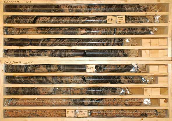
98 93 Appendix 3.10

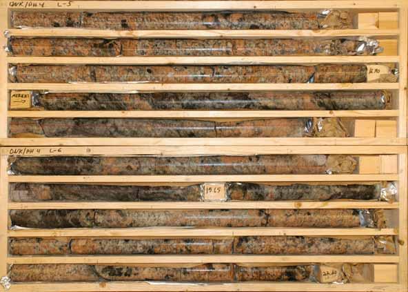
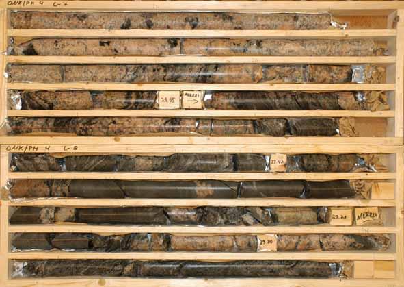
99 94

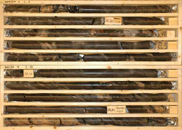
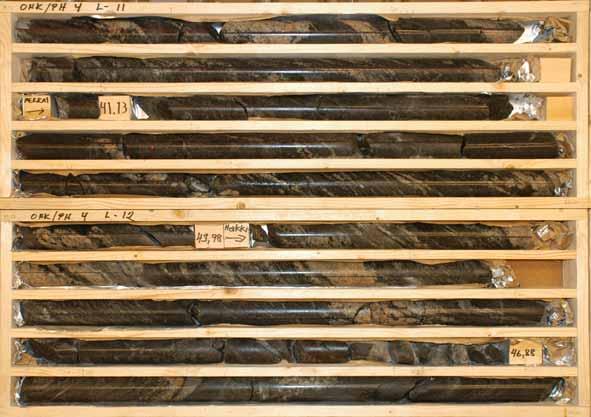
100 95

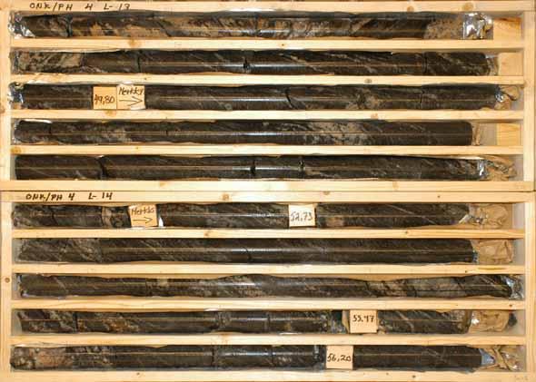
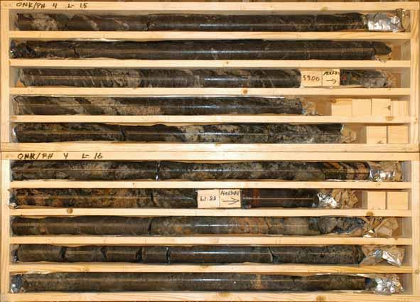
101 96

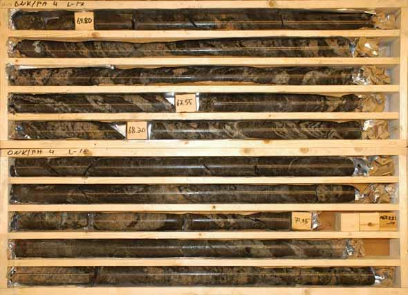
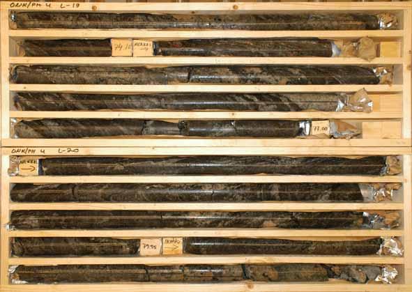
102 97

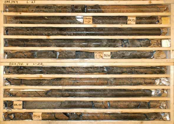
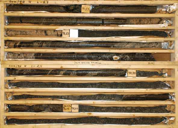
103 98

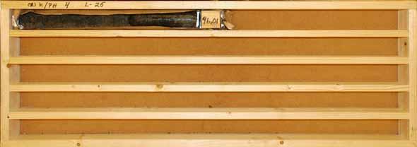
104 99

105 100

106 ROCK QUALITY Hole ID: ONK-PH4 Contractor: KATI Northing: Drilling started: Easting: Drilling ended: Elevation: Machine/fixture: ONRAM 1000/4 Direction: 315 Target: Verifing geological properties in the ONKALO profile (current layout). Dip: Purpose: Verification of geology Core diameter: 50.2 Extension: Casing: 1.5 Logging date: Remarks: PL Geologist: TJUU Max depth: HOLE_ID M_FROM M_TO LENGTH_M > 10 cm RQD RQD Jn Jr Jr Ja ROCK_QUALITY_CLASS CLASS_OF_THE Core loss REMARKS GSI cm % >10 median Profile median Q' FRACTURED_ZONE (m) Q' Q' ONK-PH PRO 1 Very Good ONK-PH URO 1 Very Good ONK-PH URO 2.5 Good ONK-PH URO 2.5 Good ONK-PH SRO 0.75 Exceptionally Good No fractures ONK-PH URO 2 Extremely Good ONK-PH URO 3 Good ONK-PH URO 1 Good RiIII ONK-PH URO 1 Very Good ONK-PH PRO 2 Good RiIII 10 l/min ONK-PH URO 1 Very Good ONK-PH URO 1 Very Good ONK-PH URO 1 Good ONK-PH URO 2 Good ONK-PH URO 1 Extremely Good ONK-PH URO 2 Good ONK-PH URO 2.5 Good ONK-PH URO 2 Very Good ONK-PH URO 3 Good ONK-PH URO 1 Extremely Good ONK-PH URO 4 Good RiII ONK-PH l/min ONK-PH URO 4 Fair RiII ONK-PH URO 6 Good Graphite and sulphid ONK-PH URO 3 Good RiIII ONK-PH URO 4 Good Graphite and sulphid ONK-PH URO 2 Extremely Good 0.15 In the beginning of th GSI=9lnQ' APPENDIX 4.1

107 102

108 103 Appendix 5.1 Olkiluoto, ONKALO, Borehole PH4 Flow rate and single point resistance Flow from the measured section (L = 0.5 m, dl = 0.1 m), Fracture specific flow (into the hole) Fracture specific flow (into the bedrock) Length (m) Flow rate (ml/h) Single point resistance (ohm)

109 104 Appendix 5.2 Olkiluoto, ONKALO, Borehole PH4 Flow rate and single point resistance Flow from the measured section (L = 0.5 m, dl = 0.1 m), Fracture specific flow (into the hole) Fracture specific flow (into the bedrock) Length (m) Flow rate (ml/h) Single point resistance (ohm)

110 105 Appendix 5.3 Olkiluoto, ONKALO, Borehole PH4 Flow rate and single point resistance Flow from the measured section (L = 0.5 m, dl = 0.1 m), Fracture specific flow (into the hole) Fracture specific flow (into the bedrock) Length (m) Flow rate (ml/h) Single point resistance (ohm)

111 106 Appendix 5.4 Olkiluoto, ONKALO, Borehole PH4 Flow rate and single point resistance Flow from the measured section (L = 0.5 m, dl = 0.1 m), Fracture specific flow (into the hole) Fracture specific flow (into the bedrock) Length (m) Flow rate (ml/h) Single point resistance (ohm)

112 107 Appendix 5.5 Olkiluoto, ONKALO, Borehole PH4 Plotted transmissivity and hydraulic aperture of detected fractures 0 Hydraulic aperture of fracture (mm) Transmissivity of fracture Length (m) Hydraulic aperture of fracture (mm) 1E-010 1E-009 1E-008 1E-007 1E-006 Transmissivity (m 2 /s) 1E-005 1E-004

113 108 Appendix 5.6 Hole: PH4 Elevation of the top of the hole (masl): Inclination: Length from the top of the hole to the fracture (m) Flow (ml/h) Fracture elevation (masl) Drawdown (m) T (m2/s) Hydraulic aperture of fracture (mm) Comments E * E * E E * E E * E E E E E E E E E E E * E E * E E E E E E * * = Uncertain i.e. the flow rate is less than 30 ml/h or the flow anomalies are overlapping or they are unclear because of noise.

114 109 Appendix 5.7 Olkiluoto, ONKALO, Borehole PH4 Electric conductivity of borehole water During flow logging, upwards (L = 0.5 m, dl = 0.1 m), Length (m) Electric conductivity (S/m, 25 o C)

115 110 Appendix 5.8 Olkiluoto, ONKALO, Borehole PH4 Temperature of borehole water During flow logging, upwards (L = 0.5 m, dl = 0.1 m), Length (m) Temperature ( o C)

116 111 Appendix 5.9 Olkiluoto, ONKALO, Borehole PH4 Flow rate out from the borehole during flow logging Flow rate out from the borehole (L/min) / 9: / 12: / 15: / 18:00 Year-Month-Day / Hour:Minute / 21: / 0:00

117 Appendix Pauli Syrjänen Object: ONKALO Access Tunnel Chainage: 895 Notes: TunnustEsi-injekJälki-injeKontroMuu poraus Drilling Type: Pilot Hole PH4 Dry Minor NormalPlentifull Hole Depth [m] Measuring Mid Depth water Ground- Water Penetration Length Pressure Measuring Time 10 min [m] [m] [bar] [bar] Mean Value Standard dev. [Lug] Interpretated Value Notes ,80 6,4 7,91 0 0,9 1,1 1,2 0,8 [l] 0,00 0,02 0,02 0,03 0,07 [Lug] 0,027 0,025 0, ,00 12,5 7, ,8 0,4 0 [l] 0,00 0,00 0,01 0,01 0,00 [Lug] 0,004 0,006 0, , ,88 18,5 24,5 8,03 8, ,3 0,3 0 [l] 0,00 0,00 0,00 0,01 0,00 [Lug] 8,9 14,2 19,6 11,5 16,9 [l] 0,79 0,35 0,28 0,28 1,50 [Lug] 0,002 0,003 0,00 0,642 0,527 0, APPENDIX 5.10 PH4_Appendices_5-10, 5-13.xls

118 Appendix Pauli Syrjänen TunnustEsi-injekJälki-injeKontroMuu poraus Dry Minor NormalPlentifull Object: ONKALO Access Tunnel Drilling Type: Pilot Hole PH4 Chainage: 895 Notes: Hole Depth [m] Measuring Mid Depth water Ground- Water Penetration Length Pressure Measuring Time 10 min [m] [m] [bar] [bar] Mean Value Standard dev. [Lug] Interpretated Value Notes ,00 30,5 8, ,8 55,4 44,2 23,1 [l] 0,45 0,60 0,78 1,08 2,08 [Lug] 0,998 0,648 2, ,00 36,6 8,21 0,5 9,3 12 3,3 1,8 [l] 0,05 0,23 0,17 0,08 0,17 [Lug] 0,139 0,074 0, , ,00 42,6 48,6 8,27 8,33 15,7 18,1 25,4 14,3 7 [l] 1,51 0,45 0,36 0,35 0,67 [Lug] 6,7 15,3 29,6 20,6 13,7 [l] 0,67 0,38 0,42 0,51 1,37 [Lug] 0,670 0,489 0,40 0,671 0,405 0, APPENDIX 5.11 PH4_Appendices_5-11, 5-14.xls

119 Appendix Pauli Syrjänen TunnustEsi-injekJälki-injeKontroMuu poraus Dry Minor NormalPlentifull Object: ONKALO Access Tunnel Drilling Type: Pilot Hole PH4 Chainage: 895 Notes: Hole Depth [m] Measuring Mid Depth water Ground- Water Penetration Length Pressure Measuring Time 10 min [m] [m] [bar] [bar] Mean Value Standard dev. [Lug] Interpretated Value Notes ,00 60,6 8,45 6,2 18,2 34,7 14,7 7 [l] 0,67 0,46 0,50 0,37 0,75 [Lug] 0,552 0,155 0, ,00 66,5 8,51 150,9 302,8 426, ,6 [l] 16,88 7,78 6,19 7,34 12,37 [Lug] 10,11 4,457 6, ,00 72,5 8,57 185,2 296,4 318,7 195,1 51,7 [l] 21,58 7,68 4,65 5,06 6,03 [Lug] ,00 78,2 8,63 210,4 399,5 423,4 220,9 86,9 [l] 25,54 10,45 6,20 5,78 10,55 [Lug] 8,999 7,131 5,00 11,70 8,059 6, ,46 86,8 8,71 182, ,7 394,5 192,7 [l] 5,010 2,653 2,50 7,66 3,34 2,53 3,40 8,11 [Lug] 114 APPENDIX 5.12 PH4_Appendices_5-12, 5-15.xls

120 Interpretation Appendix 5.13 Kuvia käytetään veden virtauksen tulkinnassa. Tulkitut arvot vain tummansinisiin soluihin. A. C. Houlsby: Construction and Design of Cement Grouting. A1990. Wiley-Interscience publication. Similar Lugeon values for each run indicates laminar flow => Use mean Lugeon value Low Lugeon values at higher pressures indicates turbulent flow => Use lowest Lugeon value High Lugeon values at higher pressures indicates dilation => Use lowest Lugeon value or medium value, if lowest values indicates turbulent flow Lugeon values increasing even when pressure drops, indicates washout => Use Lugeon value of the final run Decreasing Lugeon values throughout the test indicate void filling => Use lowest Lugeon value Groundwater Pressure Water Penetration Test Measuring Time 10 min Interpretation [bar] Pressure [bar] [Lug] 0,000 0,020 0,040 0,060 0, ,91 7,97 8, ,09 Pres. Diff. 2,09 7,09 12,09 7,09 2,09 [bar] Flow 0 0,9 1,1 1,2 0,8 [l] Penetration 0,000 0,022 0,016 0,029 0,066 [Lug] 0,02 Pres. Diff. 2,03 7,03 12,03 7,03 2,03 [bar] Flow 0 0 0,8 0,4 0 [l] Penetration 0,000 0,000 0,011 0,009 0,000 [Lug] 0 Pres. Diff. 1,97 6,97 11,97 6,97 1,97 [bar] Flow 0 0 0,3 0,3 0 [l] Penetration 0,000 0,000 0,004 0,007 0,000 [Lug] 0 Pres. Diff. 1,91 6,91 11,91 6,91 1,91 [bar] Flow 8,9 14,2 19,6 11,5 16,9 [l] Penetration 0,792 0,349 0,280 0,283 1,504 [Lug] 0,3 0,000 0,002 0,004 0,006 0,008 0,010 0,012 0,000 0,002 0,004 0,006 0,008 0,000 0,500 1,000 1,500 2, APPENDIX 5.13

121 Interpretation Appendix 5.14 Kuvia käytetään veden virtauksen tulkinnassa. Tulkitut arvot vain tummansinisiin soluihin. A. C. Houlsby: Construction and Design of Cement Grouting. A1990. Wiley-Interscience publication. Similar Lugeon values for each run indicates laminar flow => Use mean Lugeon value Low Lugeon values at higher pressures indicates turbulent flow => Use lowest Lugeon value High Lugeon values at higher pressures indicates dilation => Use lowest Lugeon value or medium value, if lowest values indicates turbulent flow Lugeon values increasing even when pressure drops, indicates washout => Use Lugeon value of the final run Decreasing Lugeon values throughout the test indicate void filling => Use lowest Lugeon value Groundwater Pressure Water Penetration Test Measuring Time 10 min Interpretation [bar] Pressure [bar] [Lug] 0,000 0,500 1,000 1,500 2,000 2, ,15 8,21 8, ,33 Pres. Diff. 1,85 6,85 11,85 6,85 1,85 [bar] Flow 5 24,8 55,4 44,2 23,1 [l] Penetration 0,450 0,603 0,779 1,075 2,081 [Lug] 2 Pres. Diff. 1,79 6,79 11,79 6,79 1,79 [bar] Flow 0,5 9,3 12 3,3 1,8 [l] Penetration 0,047 0,228 0,170 0,081 0,168 [Lug] 0,1 Pres. Diff. 1,73 6,73 11,73 6,73 1,73 [bar] Flow 15,7 18,1 25,4 14,3 7 [l] Penetration 1,513 0,448 0,361 0,354 0,675 [Lug] 0,4 Pres. Diff. 1,67 6,67 11,67 6,67 1,67 [bar] Flow 6,7 15,3 29,6 20,6 13,7 [l] Penetration 0,669 0,382 0,423 0,515 1,368 [Lug] 0,4 0,000 0,050 0,100 0,150 0,200 0,250 0,000 0,500 1,000 1,500 2,000 0,000 0,500 1,000 1, APPENDIX 5.14

122 Interpretation Appendix 5.15 Kuvia käytetään veden virtauksen tulkinnassa. Tulkitut arvot vain tummansinisiin soluihin. A. C. Houlsby: Construction and Design of Cement Grouting. A1990. Wiley-Interscience publication. Similar Lugeon values for each run indicates laminar flow => Use mean Lugeon value Low Lugeon values at higher pressures indicates turbulent flow => Use lowest Lugeon value High Lugeon values at higher pressures indicates dilation => Use lowest Lugeon value or medium value, if lowest values indicates turbulent flow Lugeon values increasing even when pressure drops, indicates washout => Use Lugeon value of the final run Decreasing Lugeon values throughout the test indicate void filling => Use lowest Lugeon value Groundwater Pressure Water Penetration Test Measuring Time 10 min Interpretation [bar] Pressure [bar] [Lug] 0,000 0,200 0,400 0,600 0, ,45 8,51 8, ,63 Pres. Diff. 1,55 6,55 11,55 6,55 1,55 [bar] Flow 6,2 18,2 34,7 14,7 7 [l] Penetration 0,667 0,463 0,501 0,374 0,753 [Lug] 0,5 Pres. Diff. 1,49 6,49 11,49 6,49 1,49 [bar] Flow 150,9 302,8 426, ,6 [l] Penetration 16,881 7,776 6,187 7,345 12,373 [Lug] 6 Pres. Diff. 1,43 6,43 11,43 6,43 1,43 [bar] Flow 185,2 296,4 318,7 195,1 51,7 [l] Penetration 21,584 7,683 4,647 5,057 6,025 [Lug] 5 Pres. Diff. 1,37 6,37 11,37 6,37 1,37 [bar] Flow 210,4 399,5 423,4 220,9 86,9 [l] Penetration 25,542 10,448 6,205 5,777 10,549 [Lug] 6 0,000 5,000 10,000 15,000 20,000 0,000 5,000 10,000 15,000 20,000 25,000 0,000 5,000 10,000 15,000 20,000 25,000 30, APPENDIX 5.15

123 Interpretation Appendix ,000 2,000 4,000 6,000 8,000 10, ,71 Pres. Diff. 1,29 6,29 11,29 6,29 1,29 [bar] Flow 182, ,7 394,5 192,7 [l] Penetration 7,664 3,343 2,533 3,399 8,110 [Lug] 2,5 118 APPENDIX 5.15

124 119 Appendix 6.1 Borehole Logging Suomen Malmi Oy P.O. Box 10 FI ESPOO Client: Posiva Oy Hole no: ONK-PH04 Ø: 76 Surveyed by:as, LJ, JM Site: Olkiluoto X: Length: 91.6 Survey date: Project no: Y: Azimuth: 315 Reported by: JM Z: Dip: Report date: Nov 2005 Lith. Fr. freq. 0 1/m 15 Depth Tunnel Chainage (m) Gamma-Gamma Density 2.6 g/cm3 3.2 Wenner Resistivity 0.2 Ohm.m 2000 Velocity P 0.6 m 4000 m/s 7000 Core loss Ri 1m:500m Susceptibility 0 1E-5 SI 1000 Natural Gamma Single Point Resistance 2 Ohm Short Normal 16" Resistivity Velocity S 0.6m 2000 m/s µr/h Ohm.m Long Normal 64" Resistivity 1 Ohm.m Radar First Wave Time 60 ns 45 Radar First Wave Ampl Veined gneiss µv Quartz gneiss Diatexitic gneiss 10.0 Pegmatite/ Pegmatitic granite Diatexitic gneiss Mafic gneiss Diatexitic gneiss 30.0 Veined gneiss Veined gneiss 40.0 Diatexitic gneiss Veined gneiss Diatexitic gneiss 60.0 Pegmatite/ Pegmatitic granite Veined gneiss 940 0

125 120 Appendix 6.1 Veined gneiss Diatexitic gneiss 70.0 Veined gneiss Pegmatite/ Pegmatitic granite 80.0 Pegmatite/ Pegmatitic granite Veined gneiss 970 0

126 121 Appendix 6.2 Borehole Radar Suomen Malmi Oy P.O. Box 10 FI ESPOO Client: Posiva Oy Hole no: ONK-PH04 Ø: 76 Surveyed by:jm, AS; LJ Site: Olkiluoto X: Length: 91.6 Survey date: Project no: Y: Azimuth: 315 Reported by: JM Z: Dip: Report date: Nov 2005 Lith. Fr. freq. Depth Tunnel Single Point Resistance Radar Raw Image, 250 MHz 0 1/m 15 Core 1m:500m Chainage 1 Ohm Radar First Wave Time 30 Nanosecond 200 loss Ri 60 ns 45 Radar First Wave Ampl Veined gneiss µv Quartz gneiss Diatexitic gneiss 10.0 Pegmatite/ Pegmatitic granite Diatexitic gneiss Mafic gneiss Diatexitic gneiss 30.0 Veined gneiss Veined gneiss 40.0 Diatexitic gneiss Veined gneiss Diatexitic gneiss 60.0 Pegmatite/ Pegmatitic granite Veined gneiss Diatexitic gneiss 70.0 Veined gneiss

127 122 Appendix 6.2 Pegmatite/ Pegmatitic granite Pegmatite/ Pegmatitic granite Veined gneiss 970 0

128 Borehole Radar Suomen Malmi Oy P.O. Box 10 FI ESPOO Client: Posiva Oy Hole no: ONK-PH04 Ø: 75.7 Surveyed by:jm, AS, LJ Site: Olkiluoto X: Length: 91.6 Survey date: Project no: Y: Azimuth: 315 Reported by:jm Z: Dip: Report date: Sept Lith. Fr. freq. 0 1/m Core loss Ri 15 Depth 1m:200m Tunnel Chainage Fract.Angles degrees 0 90 Radar Intersect Angle 0 90 Orient. Reflect. degrees 0 90 Oriented fract. degrees 0 90 Radar Orientations Schmidt Plot - Lower Hemisphere Refl. ext. bckwd 15 m 0 Refl. ext. fwd 0 m 15 Range out 0 m 15 Veined gneiss Quartz gneiss Diatexitic gneiss Pegmatite/ Pegmatitic granite Schmidt Plot - Lower Hemisphere Depth: [m] to [m] Mean Counts Dip[deg] Azi[deg] Appendix 6.3

129 Schmidt Plot - Lower Hemisphere Depth: [m] to [m] Diatexitic gneiss Mafic gneiss 28.0 Mean Counts Dip[deg] Azi[deg] Diatexitic gneiss Veined gneiss Veined gneiss Diatexitic gneiss Schmidt Plot - Lower Hemisphere Depth: [m] to [m] Mean Counts Dip[deg] Azi[deg] Appendix 6.3

130 48.0 Veined gneiss 52.0 Schmidt Plot - Lower Hemisphere Depth: [m] to [m] Diatexitic gneiss 60.0 Mean Counts Dip[deg] Azi[deg] Pegmatite/ Pegmatitic granite Veined gneiss Diatexitic gneiss Veined gneiss Schmidt Plot - Lower Hemisphere Depth: [m] to [m] Mean Counts Dip[deg] Azi[deg] Appendix 6.3

131 80.0 Pegmatite/ Pegmatitic granite Pegmatite/ Pegmatitic granite 84.0 Schmidt Plot - Lower Hemisphere Depth: [m] to [m] Veined gneiss 92.0 Mean Counts Dip[deg] Azi[deg] Appendix 6.3

132 Ext. backward Ext. forward Range out CLASS Comment FILTER TYPE Nr. Depth Angle Azimuth Dip L-45-nftunnfront PLANE not oriented tunnel front? No Filter PLANE L-46-nf not oriented not known No Filter PLANE L-41-nf not oriented not known No Filter PLANE L-50-nf Fract 4.15 No filter PLANE L-47-nf Fract 4.25 No Filter PLANE L-43-nf Delay. Conductive. FOL; one possibility of No Filter PLANE L-90-HFIR FOL HFIR PLANE L-48-nf not oriented not known NoFilter PLANE L-40-nf not oriented not known NoFilter PLANE L-49-nf Fract 9.85 NoFilter PLANE L-44-nf-attdel-stro Strong, Conductive. Attenuation and delay Fract 10.06, gentler dip No Filter PLANE L-39-nfstrong Strong. Attenuation and delay. fract 11.51, gentler NoFilter PLANE L-91-HFIR not oriented not known HFIR L-38-nfstrong fract in , not PLANE Strong accurate No Filter PLANE L-51-nf fract in , not accurate No Filter PLANE L-34-nf may fit at 14.8 fract No Filter PLANE L-92-FIR may fit at fract FIR PLANE L-42-nf fractures 16.9 NoFilter PLANE L-93-HFIR- Strong strong fractures 17.31, gentler HFIR PLANE L-37-nf not oriented not known No Filter PLANE L-33-nf not oriented not known No Filter PLANE L-35-nf not oriented not known No Filter PLANE L-32-nf not oriented not known No Filter 127 Appendix 6.4

133 PLANE L-53-nf not oriented not known No Filter fracture at No Filter PLANE L-54-nf fracture at No Filter PLANE L-36-nf fracture 25.38, No Filter PLANE L-52-nf steeper? PLANE L-57-nf fracure No Filter PLANE L-94-FHIRstrong strong. conductive, attenuation, delay. fractures 27.12, concord. fol HFIR PLANE L-95-HFIR Edge of cond. fract HFIR fract 28.38, PLANE L-59-nf slicknsd No Filter PLANE L-89-FIR fract FIR PLANE L-31-nf fract No Filter PLANE L-28-nf fract 29.5 No Filter PLANE L-56-nf fract No Filter PLANE L-29-nf not oriented not known No Filter PLANE L-55-nf Delay. fract at No Filter fract orient at No Filter PLANE L-27-nf PLANE L-30-nf fol orient No Filter PLANE L-58-nf foliation No Filter PLANE L-88-FIR foliation FIR PLANE L-87-FIR Attenuation Conductive. fracture FIR Attenuation. No Filter PLANE L-26-nf Conductive. fracture fract 37.48, No Filter PLANE L-60-nf orient from fol PLANE L fol No Filter PLANE L-22-nf fract No Filter Strong. Attenuation. PLANE L-86_FIR Conductive. Delay. fract 41.36, orient from fol FIR PLANE L-85-FIR fol FIR 128 Appendix 6.4

134 PLANE L-18-nf fol or fract. No Filter PLANE L-96_HFiR not oriented not known HFIR PLANE L-15-nf not oriented not known No Filter PLANE L-61-nf fract 44.48, gentler? No Filter PLANE L-62-nf fol No Filter PLANE L-20-nf not oriented not known No Filter foliation and PLANE L-84-FIR PLANE L-21-nf PLANE L-81-IR PLANE L-63-nf fracture 46.1 foliation and fracture 46.1 FIR NoFilter Strong. Attenuation. Delay. conductive. fracture FIR Strong. Attenuation. Delay. conductive. Strong. Attenuation. Delay. conductive. foliation, gentler dip No Filter fracture at PLANE L No Filter foliation at 48- PLANE L-24-nf No Filter PLANE L-83-FIR fract at FIR PLANE L-82-FIR not oriented not known FIR PLANE L-23-nf foliation No Filter PLANE L-76-FIR foliation FIR PLANE L-80-FIR foliation FIR PLANE L-97-hfir PLANE L possible fracture fol or fract at 53, orient from fol HFIR No Filter PLANE L Strong. fol or fract at 53.12, orient from fol No Filter PLANE L-16-NF strong fract at No Filter 129 Appendix 6.4

135 strong PLANE L-79-FIR- Strong strong fract at FIR PLANE L-73-FIR fract at FIR PLANE L fract at No Filter PLANE L-13-nf fract at No Filter PLANE L-12-nfstrong strong fol No Filter PLANE L fract at No Filter L-9-NF-attdel-60m attenuation and time PLANE delay fol No filter PLANE L-10-nf-attdel-stro PLANE L-74-FIR PLANE L-6-NF PLANE L-8-nfcondhangwall PLANE L-71-FIR attenuation, time delay, strong fract No Filter strong att., cond fol FIR fractures 62.50, strong att., closest not cond. oriented No Filter conductive zone, hanging wall fractures 63.2 NoFilter almost total attenuation. fracture FIR almost total att. fractures 65.0 No Filter PLANE L-7-nf PLANE L-69-FIR fracture FIR PLANE L-5-NF fol No filter PLANE L-75-FIR strong fracture 68.4 FIR PLANE L-77-FIR fracture 68.4 FIR PLANE L-4-NF- CoHangWall- Str PLANE L-70-FIR Strong. Conductive zone hanging wall. fracture No filter almost total attenuation, very conductive. fracture 71.05, or conductive zone. FIR 130 Appendix 6.4

136 PLANE PLANE PLANE conductive, almost toatal PLANE L-3-NF- Cond-Att-Del not oriented attenuation, time delay not known No Filter PLANE L-68-FIR not oriented not known FIR PLANE L-66-FIR not oriented edge of attenuated zone not known FIR PLANE L foliation No Filter PLANE L-64-nf foliation No filter PLANE L-67-FIR fracture FIR L-98-HFIR- Stro not oriented strong not known HFIR L-1-NF- bottom of Bottom not oriented open section not known No Filter fract 81.5, L-65-nfstrong orientation from strong No filter PLANE L-78-FIR not oriented does not intersect, apparent location FIR 131 Appendix 6.4

137 132 Appendix

138 133 Appendix 6.5

139 134 Appendix 6.6 Acoustic Logging Suomen Malmi Oy P.O. Box 10 FI ESPOO Client: Posiva Oy Hole no: ONK-PH04 Ø: 76 Surveyed by:jm, AS, LJ Site: Olkiluoto X: Length: 91.6 Survey date: Project no: Y: Azimuth: 315 Reported by: JM Z: Dip: Report date: Nov 2005 Lith. Fr. freq. Depth Tunnel Velocity P 0.6 m Apparent Q Poisson's Ratio P Attenuation Tubewave En. R1 0 1/m 15 Core 1m:500m Chainage 4000 m/s 7000 Velocity P 1m G-G Density Shear Modulus -100 db/m 100 S Attenuation Tubewave En. R2 loss Ri 4000 m/s 7000 Velocity S 0.6m 2.6 g/cm GPa 50 Young's Modulus -100 db/m Tubewave Attenuation 2000 m/s GPa db/m 30 Velocity S 1m Bulk Modulus 2000 m/s GPa 200 Bulk Compr 0 1/GPa 0.1 Veined gneiss 0.0 Quartz gneiss Diatexitic gneiss 10.0 Pegmatite/ Pegmatitic granite Diatexitic gneiss Mafic gneiss Diatexitic gneiss 30.0 Veined gneiss Veined gneiss 40.0 Diatexitic gneiss Veined gneiss Diatexitic gneiss 60.0 Pegmatite/ Pegmatitic granite Veined gneiss 940.0

140 135 Appendix 6.6 Diatexitic gneiss 70.0 Veined gneiss Pegmatite/ Pegmatitic granite 80.0 Pegmatite/ Pegmatitic granite Veined gneiss 970.0

141 136 Appendix 6.7 Acoustic Logging Suomen Malmi Oy P.O. Box 10 FI ESPOO Client: Posiva Oy Hole no: ONK-PH04 Ø: 76 Surveyed by:jm, AS, LJ Site: Olkiluoto X: Length: 91.6 Survey date: Project no: Y: Azimuth: 315 Reported by:jm Z: Dip: Report date: Nov 2005 Lith. Fr. freq. Depth Tunnel Velocity P 0.6 m Full Wave Sonic, 0.6 m Full Wave Sonic, 1 m 0 1/m 15 Core 1m:500m Chainage 4000 m/s 7000 Velocity S 0.6m 0 µs µs 2048 loss Ri 2000 m/s 4000 Veined gneiss 0.00 Quartz gneiss Diatexitic gneiss Pegmatite/ Pegmatitic granite Diatexitic gneiss Mafic gneiss Diatexitic gneiss Veined gneiss Veined gneiss Diatexitic gneiss Veined gneiss Diatexitic gneiss Pegmatite/ Pegmatitic granite Veined gneiss Diatexitic gneiss Veined gneiss

142 137 Appendix 6.7 Pegmatite/ Pegmatitic granite Pegmatite/ Pegmatitic granite Veined gneiss 970 0

143 Borehole Imaging 138 Appendix 6.8 Suomen Malmi Oy P.O. Box 10 FI ESPOO Client: Posiva Oy Hole no: ONK-PH04 Ø: 76 Surveyed by: JM, AS Site: Olkiluoto X: Length: 91.6 Survey date: Project no: Y: Azimuth: Reported by: JM Z: Dip: Report date: Nov 2005 Depth 1m:2m 1.50 ONK-PH04 3-D Image 0 ONK-PH04 Image Section 0-41 m Oriented to North (0º), Depth Adjusted

144

145 140 Appendix 6.9

146 141 Appendix 6.9

147 142 Appendix 6.10 Rautaruukki RROM-2 Specifications Antenna dimensions -diameter 42 mm -length 1570 mm -electrode separation a=318 mm -diameter of the electrodes 40 mm Measuring cable minimum 4-conductor, length up to 1000 m, loop resistance for output voltage conductors max 40 Ohm Measuring current 10 ma/20 Hz Range Ohm-m Output voltage +5 V -6 V Power feed 18 V, 3 Ah Power consumption 2.4 W Operation temperature C

148 Logging Sondes 143 Appendix 6.11 Normal Resistivity Sonde The Geovista digital Normal Resistivity Sonde can be used on its own or in combination with other Geovista sondes for efficient logging and correlation purposes. The SP can be recorded with the sonde either powered on or off, using the 16 electrode and a surface fish. Specifications: Weight Length Diameter 64 N & 16 N Resistivity Range SPR SP Range Current return Measure return Max. Pressure 8kg 2.27m 42mm 1 to 10,000 Ohmm 1 to 10,000 Ohm -2.5V to +2.5V Cable armour Bridle electrode 20MPa Max. Temperature 80ºC Focused Resistivity Sonde Provides resistivity logs with finer vertical resolution and a deeper depth of investigation. Performance is best in higher conductivity mud and higher resistivity formations. The probe can be used on its own or in combination with other Geovista sondes. Specifications: Weight 7.0 kg Length 2.37m Diameter Range Max. Pressure 38mm 1 to 10,000 Ohmm 20MPa Max. Temperature 80ºC Geovista reserve the right to change the products list and specifications without prior notice UNIT 6,CAE FFWT BUSINESS PARK,GLAN CONWY, LL28 5SP,UK WEB SITE: PHONE: +44 (0) FAX: +44 (0) geovista@geovista.co.uk

149 144 Appendix 6.12 Introduction to RAMAC/GPR borehole radar MALÅ GeoScience

150 INTRODUCTION 145 Appendix 6.12 Borehole radar is based on the same principles as ground penetrating radar systems for surface use, which means that it consists of a radar transmitter and receiver built into separate probes. The probes are connected via an optical cable to a control unit used for time signal generation and data acquisition. The data storage and display unit is normally a Lap Top computer, which is either a stand-alone component or is built into the circuitry of the control unit. Borehole radar instruments can be used in different modes: reflection, crosshole, surface-to-borehole and directional mode. Today s available systems use centre frequencies from 20 to 250 MHz. Radar waves are affected by soil and rock conductivity. If the conductivity of the surrounding media is more than a certain figure reflection radar surveys are impossible. In high conductivity media the radar equation is not satisfied and no reflections will appear. In crosshole- and surface-to-borehole radar mode measurements can be carried out in much higher conductivity areas because no reflections are needed. Important information concerning the local geologic conditions are evaluated from the amplitude of the first arrival and the arrival time of the transmitted wave only, not a reflected component. Common borehole radar applications include: Geological investigations Engineering investigations Environmental investigations Hydropower dams investigations Fracture detection Cavity detection Karstified area investigation Salt layers investigations DIPOLE REFLECTION SURVEYS In reflection mode the radar transmitter and receiver probes are lowered in the same borehole with a fixed distance between them. See figure 1. In this mode an optical cable for triggering of the probes and data acquisition is necessary to avoid parasitic antenna effects of the cable. The most commonly

151 146 Appendix 6.12 used antennas are dipole antennas, which radiate and receive reflected signals from a 360-degree space (omnidiretionally). Borehole radar interpretation is similar to that of surface GPR data with the exception of the space interpretation. In surface GPR surveys all the reflections orginate from one half space while the borehole data receive reflections from a 360- degree radius. It is impossible to determine the azimuth to the reflector using data from only one borehole if dipole Figure 1 antennas are used. What can be determined is the distance to the reflector and in the case where the reflector is a plane, the angle between the plane and the borehole. As an example, let s imagine a fracture plane crossing a borehole and a point reflector next to the same borehole (figure 1, left). When the probes are above the fracture reflections from the upper part of the plane are imaged, in this case from the left side of the borehole. When the probes are below the plane, reflections from the bottom of the plane are imaged, in this case the right side of the borehole. The two sides of the plane are represented in the synthetic radargram in figure 1. They are seen as two legs corresponding to each side of the plane. When interpreting borehole radar data, it is important to remember that the radar image is a 360-degree representation in one plane. A point reflector shows up as a hyperbola, in the same way as a point reflector appears in surface GPR data.interpreting dipole radar data from a single borehole, the interpreter can not give the direction to the point reflector only the distance to source can be interpreted. In order to estimate the direction to the reflection, data from more than one borehole need to be interpreted. Figure 2: Dipole reflection measurement in granite. The antenna centre frequency used was 100 MHz. In granite, normally several tens of meters of range are achieved using this antenna frequency.

152 147 Appendix 6.13 Full Waveform Sonic Tool The ALT full waveform sonic tool has been specially designed for the water, mining and geotechnical industries. Its superior specification makes it ideal for a cement bond logs, for the measurement of permeability index, and as a specialist tool to carry out deep fracture identification. TECHNICAL SPECIFICATIONS OD: 50 or 68mm Length: variable depending on configuration Max pressure: 200 bars Max temperature: 70 C Variable spacing: all traces synchronously and simultaneously recorded Frequency of sonic wave: 15KHz Sonic wave sampling rate: configurable, 2 usec -> 50 µsec Sonic wave length: configurable, up to 1024 samples per receiver Dynamic range: 12 bits plus configurable 4 bits gain incl. AGC Data communication: compatible with ALT acquisition system Required wireline: single or multi- conductors Modular tool allowing a configuration of up to 2 transmitters and 8 receivers Advantages of the tool include : High energy of transmission to give a greater depth of penetration or longer spacings. Lower frequency of operation for greater penetration, especially for the CBL. Ability to record a long wave train for Tube wave train reflection wich allows for the measurement of fracture aperture and permeability index. The absolute value of the amplitude of the received wave form is measurable thus allowing for the calibration of the amplitude. Truly modular construction allowing variation of receiver/transmitter combinations. Higher logging speeds when used in conjunction with the ALT Logger acquisition system due to the superior rate of data communication possible.

153 148 Acquisition systems Appendix 6.14 ALTlogger 19 rack mountable ALTlogger minirack ABOX W L H W 48.3 cm (19 ) 50 cm (19,7 ) 13.2 cm (3U) 16-20kgs without packaging 37.6 cm (14.5 ) 35 cm (13.8 ) 13.2 cm (3U) 12-16kgs without packaging 26 cm 16 cm 9 cm 3kgs ALT s family of acquisition system is based on modern electronic design in which software control techniques have been used to the best advantage. The hardware incorporates the latest electronic components with embedded systems controlled via the specially developed ALTlogger Windows interface program. Main features high speed USB interface Self selecting AC power source from AC 100V to AC 240V Ruggedised system, heavy duty, fault tolerant Interfaces downhole probes from many manufacturer (not available on Abox system) Wireline and winch flexibility (runs on coax, mono, 4 or 7 conductor wireline) Compatible with most shaft encoder (runs on any 12V or 5V quadrature shaft encoder with any combination of wheel circumference/shaft pulse per revolution) Totally software controlled Very easy to use, with graphical user interface (dashboard), self diagnostic features, configurable through files and minimal technical knowledge needed from the user Runs on any notebook PC compatible Windows 2000 & windows XP. Real time data display and printing Supports Windows supported printers and Printrex thermal printers optional network enabled distributed architecture ALTlogger 19 rack and minirack The rack system has been designed to accommodate multivendor tool types. The modular and flexible design architecture of the system will allow virtually any logging tool to run on any winch supposed the required Tool Adapter and Depth Encoder Adapter is inserted into the ALTlogger Unit. Any new combination of logging tool and winch unit will just require selection of the proper ALTlog.ini File and the proper Tol-File. The Tool Adapter is the software and hardware suitable to interface a specific family of tools. It provides the interface between a tool specific power, data protocol and wireline conductor format and the system core. When a logging tool is selected for use, the system automatically addresses the type of adapter associated with the tool. The latest Digital Signal Processing (DSP) adapter adds even more flexibility to the system with expansion slots for future developments and upgrades, by implementing a 100% firmware based modem system. The specifications are not contractual and are subject to modification without notice.

154 149 Appendix 6.14 The acquisition system ALTLoggersoftware runs on Windows OS and exploits the true pre-emptive multitasking ability of the Windows NT Kernel Dashboard The heart of the graphical user interface is called the Dashboard and consists of multiple threads running concurrently and handling specific system tasks. The dashboard is also the operator s control panel. It is used to select and control all systems functions and to monitor data acquisistion. The dashboard contains seven sub windows: Depth (depth system) Tool (tool configuration & power) Communication (data flows and communication control) Acquisition (data sampling and replay controls) Browser and processors (data browser and processors controls) Status (self diagnostic system status indicators) tension (tension gauge system TOL file Information specific to a particular tool is contained in a unique tool configuration file which has the extension *.TOL. Information contained in the *.TOL file is used by different components of the system for initialising Dashboard components (tool power, data protocol, etc ), as well as setting parameters for client processes (browser & processors) handling data calibration, data processing, data display or printing. A copy of the TOL file is included in each data file acquired Browser and processors (real time data monitoring) A Browser is a Client Process. The Browser offer the operator of the logging system a number of different on-line display facilities to present log data on the screen in a user-friendly, easy controllable, attractive layout. Depending on the tool category, different Browser are used to display log data such as conventional curves, full waveform sonics, borehole images... Typical user screen with scrolling log display and data monitoring Bâtiment A, Route de Niederpallen, L-8506 Redange-sur-Attert. Grand-Duché de Luxembourg T:(352) F:(352) sales@alt.lu

155 150 Appendix 6.14 OBI 40 slimhole optical televiewer The tool generates a continuous oriented 360 image of the borehole wall using an optical imaging system. (downhole CCD camera which views a image of the borehole wall in a prism). The tool includes a orientation device consisting of a precision 3 axis magnetometer and 3 accelerometers thus allowing accurate borehole deviation data to be obtained during the same logging run (accurate and precise orientation of the image). Optical and acoustic televiewer data are complimentary tools especially when the purpose of the survey is structural analysis. A common data display option is the projection on a virtual core that can be rotated and viewed from any orientation. Actually, an optical televiewer image will complement and even replace coring survey and its associated problem of core recovery and orientation. The optical televiewer is fully downhole digital and can be run on any standard wireline (mono, four-conductor, sevenconductor). Resolution is user definable (up to 0.5mm vertical resolution and 720 pixels azimuthal resolution) Bâtiment A, Route de Niederpallen, L-8506 Redange-sur-Attert. Grand-Duché de Luxembourg T:(352) F:(352) sales@alt.lu