Monitoring Hydraulic Conductivity with HTU at Eurajoki, Olkiluoto, Drillholes OL-KR4, OL-KR8, OL-KR28 and OL-KR31 in 2006

Transkriptio

1 Working Report Monitoring Hydraulic Conductivity with HTU at Eurajoki, Olkiluoto, Drillholes OL-KR4, OL-KR8, OL-KR28 and OL-KR31 in 2006 Heikki Hämäläinen May 2007 POSIVA OY FI OLKILUOTO, FINLAND Tel Fax

2 Working Report Monitoring Hydraulic Conductivity with HTU at Eurajoki, Olkiluoto, Drillholes OL-KR4, OL-KR8, OL-KR28 and OL-KR31 in 2006 Heikki Hämäläinen Geopros Oy May 2007 Base maps: National Land Survey, permission 41/MYY/07 Working Reports contain information on work in progress or pending completion. The conclusions and viewpoints presented in the report are those of author(s) and do not necessarily coincide with those of Posiva.

3 MONITORING HYDRAULIC CONDUCTIVITY WITH HTU AT EURAJOKI, OLKILUOTO, DRILLHOLES OL-KR4, OL-KR8, OL-KR28 AND OL-KR31 IN 2006 ABSTRACT The construction of the ONKALO, may form a significant disturbance to the hydraulic properties of the Olkiluoto area. This disturbance is studied by a monitoring programme, which includes measurements of hydraulic conductivity in adjacent drillholes OL-KR4, OL-KR8, OL-KR28 and OL-KR31. The tests determining the hydraulic conductivity described in this report were performed in the early stages of the excavation of ONKALO. They provide together with previous tests a baseline to which later results can be compared. The same measurement program was first completed in 2005 and it was repeated now in Double-packer constant-head method was used throughout with 2 m packer separation and a nominal 200 kpa overpressure. Injection stage lasted normally 20 minutes and fall-off stage 10 minutes. The tests were often shortened if there were clear indications that the hydraulic conductivity was below the measuring range of the system. The pressure in the test section was let to stabilise at least 5 min before injection, occasionally longer. Also, the injection and fall-off were extended when necessary to obtain a stationary state. Two transient (Horner and 1/Q) interpretations and one stationary-state (Moye) interpretation were made in-situ immediately after the test. A total of 267 tests were accomplished covering altogether 530,32 m of borehole in these four holes. The Hydraulic Testing Unit (HTU-system) is owned by Posiva Oy and it was operated by Geopros Oy. Keywords: HTU, hydraulic conductivity, constant head test, hydraulic injection test

4 VEDENJOHTAVUUDEN MONITOROINTIMITTAUKSET HTU- LAITTEELLA EURAJOEN OLKILUODON KAIRANREI ISSÄ OL-KR4, OL- KR8, OL-KR28 JA OL-KR31 VUONNA 2006 TIIVISTELMÄ ONKALOn rakentamisen vaikutuksia Olkiluodon saaren hydraulisiin ominaisuuksiin tutkitaan, monitorointiohjelmalla, johon liittyen vedenjohtavuutta mitattiin HTU- laitteella ONKALOn lähellä olevissa kairanrei issä. Ennen tunnelin rakentamisen aloittamista ja rakentamisen alkuvaiheessa tehdyt tutkimukset muodostavat pohjatason, johon louhinnan edistyessä myöhempiä tuloksia voidaan verrata. Mittausohjelma, johon kuuluivat valitut osuudet rei istä OL-KR4, OL-KR8, OL-KR28 ja OL-KR31, toteutettiin ensimmäisen kerran 2005 ja toistettiin nyt Mittaukset tehtiin kaksoistulppa- ja vakiopainemenetelmällä käyttäen 2 m tulppaväliä ja 200 kpa ylipainetta. Injektio kesti tavallisesti 20 min ja paineenlaskuvaihe 10 min, mutta ajat vaihtelivat tilanteen mukaan. Mikäli testin aikana kävi ilmeiseksi, että vedenjohtavuus alittaa mittausalueen alarajan, sitä lyhennettiin huomattavasti. Paineen annettiin tasoittua luonnolliseen tasoonsa ennen injektiota vähintään 5 min, paikoin pidempään. Samoin injektiota jatkettiin tarpeen mukaan stationääritilan saavuttamiseksi. Vedenjohtavuudet tulkittiin välittömästi käyttäen kahta transientti- (Horner ja 1/Q) ja yhtä stationääritilan (Moye) tulkintaa. Mittauksia tehtiin yhteensä 267 kpl neljässä reiässä peittäen kaikkiaan 530,32 m pituuden kairanreikää. Mittauksissa käytettiin Posivan omistamaa HTU-laitteistoa (Hydraulic Testing Unit). Mittaukset suoritti Geopros Oy:n henkilökunta. Avainsanat: HTU, vedenjohtavuus, vakiopainekoe, vesimenekkikoe

5 1 TABLE OF CONTENTS ABSTRACT TIIVISTELMÄ 1 INTRODUCTION MEASUREMENTS EQUIPMENT General description Functional description Technical Specifications Dimensions Digital accuracy Pressure sensors Flow Transducers Temperature sensors Cable Tension Test section Depth Pressure control Single Point Resistance Measurement range Calibration TEST SEQUENCE Inflation Stabilisation Injection Fall-off SP-log Recorded variables INTERPRETATION THEORY Moye /Q Horner Sources of interpretation errors CONTENTS OF THE TEST REPORT Test information and results Diagrams Event log DATAFILE CONFIGURATION REFERENCES APPENDICES 1 Lists of tests Conductivity diagrams Map of the location Comparison of the results Test reports... on attached CD

6 2

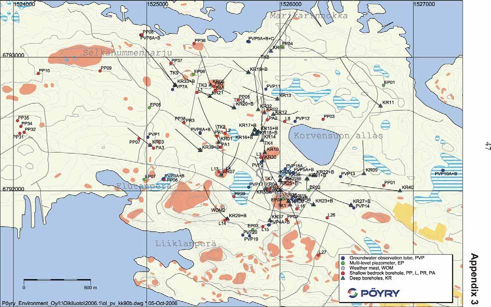
7 3 1 INTRODUCTION Posiva Oy has made investigations of the suitability of bedrock for final disposal of spent nuclear fuel at Olkiluoto, Eurajoki. After comprehensive studies a preliminary plan for an underground research facility, ONKALO, was made. ONKALO is being built near the intended rock volume for the disposal. The purpose is to explore the rock conditions at the actual repository depth and to produce detailed knowledge for the application. The length of the ONKALO tunnel will be over 5 km over a projected area of about 6 hectares. Thereby the tunnel will be a major disturbance in rock mass and may affect the groundwater conditions in the neighbourhood. The excavation can influence the conditions in many ways. As the pressure levels may change, also the flow of the groundwater may change both in rate and direction. These changes in the flow can affect the fracture fillings thereby altering the properties of aquifers. The tunnel also releases stresses in the nearby bedrock, which can cause minor deformations in adjacent structures. These deformations can influence the hydraulic conductivity significantly by changing fracture openings. Also, the blasting shocks may modify the existing fractures or strengthen the processes mentioned above. The first monitoring measurements in OL-KR4, OL-KR8, OL-KR28 and OL-KR31 in 2005 were planned to provide a baseline for monitoring the possible effects of the construction of ONKALO. There are also measurements carried out in OL-KR4 and OL-KR8 before the construction was started. The results of these measurements can be compared already with the monitoring data. The same monitoring program as in 2005 was repeated in 2006 and these results can now be compared with the one year older baseline data. The holes selected for the monitoring purpose were OL-KR4, OL-KR8, OL-KR28 and OL-KR31. They are all adjacent to the tunnel, as can be seen in Fig. 1, where they are highlighted in purple colour. The broad grey line is the tunnel. Measurements were done in one shift by a single operator. The responsible contractor was Geopros Oy. The operators were Heikki Hämäläinen and Raimo Para from Geopros Oy, Aimo Hiironen from Posiva Oy supervised the fieldwork. This report is written by Heikki Hämäläinen from Geopros Oy. Fig. 1 Location of the tunnel and holes, measured holes in purple colour.

8 4

9 5 2 MEASUREMENTS The first test was accomplished in OL-KR and continued according the times presented in Tab. 1, the last test was finished in OL-KR31 and then the HTU-system was transported to a storage area. A total of 267 measurements were performed covering the measurement plan fully. Originally OL-KR26 was included in the measurement plan, but as it was inaccessible due to ongoing reconditioning of the hole, it was replaced by KR31. A few tests were interrupted for various reasons and they have been omitted from the report. They may contain some useful information for basic studies, but in this case the conditions in the borehole can be regarded as known and that possible additional information is not relevant. Technical issues caused very few minor problems in these tests, though some such failures were encountered. The cable and the installation of the cable head were renewed in 2005 and with the new equipment there were hardly any data transmission failures. In the beginning of work in OL-KR31 the upper packer was thought to have burst, but later it was found that only the moving lower end was stuck. A spare packer was taken into use, which made the move of the tool interface from the broken packer to the spare packer necessary. Apparently the threaded connection in the upper end of the spare packer was left leaking very little due to corrosion in the threads. There are also other possible sources for the leak, but in any case the measurements in OL-KR31 contain a constant error. A steady flow of 0,015 ml/s is seen throughout the results. As almost the whole length of the hole is known to have low but measurable conductivity, it was impossible to notice the leak until the last couple of tests, where there should have been three successive tests with hydraulic conductivities below the measurement range. In addition, such leaks normally produce no, or only weak flow transients but in this case the flow transients seemed normal and they were repeatable. The leak alone equals a K-value under 2*10-10 m/s and this value should be subtracted from all results in OL-KR31. With K-values over 10-8 m/s the error is smaller than the normal noise in the measurement. In Appendix 4 a column is shown where a correction has been applied by subtracting from the K-values 1,5*10-10 m/s, which is the average value of the error. In Moye-interpretation the K-value is linear with flow and this correction is valid. The transient interpretations would require correction applied to flow data and new interpretations should be made. With the correction applied, the results show a very similar behaviour with other holes in the program. As seen already from the previous monitoring tests, which included some repeats of old tests, the measured conductivities decrease with time. Though the yearly change is not big, the tendency is continuous and evident. Fractures in the upper sections of OL-KR4 have been mostly cemented in the reconditioning of the hole and also due to the closeness of the ONKALO groutings after previous measurements. Especially sections with K-values of 1*10-9 m/s or under have become completely tight. Fractures that are more open have stayed conductive, probably because they have stronger natural flow and they are wide enough for cement particles to be flushed away. Single Point Resistance Logs from 76 mm diameter holes, i.e. OL-KR28 and OL-KR31 exist, but are not included in this report due to their small significance in the relatively low depths. Comparing the data with core observations and measurements with other

10 6 methods, the depths seem to coincide. The SPR-logs are available, if some later need arises. Tab. 1 Hole data Hole Hole depth Casing Tests performed First test Last test end OL-KR4 901,58m 39,97 m OL-KR8 600,59 m 20,10 m OL-KR28 656,33 39,98 m OL-KR31 189,88 m 40,10 m

11 7 3 EQUIPMENT 3.1 General description The equipment is described in detail in its documentation (Hämäläinen, H. 2005), in Finnish). The system consists of a pair of inflatable packers, a downhole tool, a borehole cable and a trailer, where the surface equipment is installed. The downhole tool contains pressure sensors to record the pressures in the test section, below packers and above packers, and a temperature sensor. Also, sensors for observation of eventual water leakage etc. are installed. An active pressure regulator with position indication is fitted to the injection line. The injection line opens to the test section and at higher conductivities the constant overpressure is kept by regulating the flow. There is also a bypass valve over the upper packer to equalise the pressure difference during inflation of the packers. All sensors are connected to a microprocessor controlled electronics unit, which has also got a sine wave output for the Single Point Resistance electrode. The digital data transfer between the tool and surface is in serial RS-485 format. The upper packer is attached to the tool and the lower packer is connected to it with aluminium rods. The borehole cable is custom built for this purpose. It contains polyamide hoses for injection and packer inflation and the necessary copper wire conductors. The stress member is a Kevlar webbing below the outer polyurethane jacket. The trailer is built on the chassis of a log carriage. The body is of GRP sandwich construction with polyurethane foam inner acting also as thermal insulation. A bulkhead divides the space to control and winch rooms. The controller PC, data logger, printers and power supplies are located in the control room, while the cable winch, majority of measurement and control appliances and actuators together with service facilities are in the winch room. The cable is fed to the borehole through a hatch in the floor. A hydraulic power supply, a compressor and a 500 l pressure vessel are installed below the floor. The trailer is equipped with electric heating which is capable to keep the system operational also in severe winter conditions. Fig. 2 System configuration.

12 8 3.2 Functional description The system is primarily designed for constant head injection tests, but several other types of tests are possible with minor software modifications. The tool and the cable are dimensioned for operation down to 1020 m depth. The minimum hole diameter is 56 mm, and wider holes just need a suitable set of packers. The measurement range is 1*10-4 to 1*10-11 m/s based on Moye interpretation and 2 m packer separation. The range of the flow measurement is 0, ml/s (3,6 ml/h to 468 l/h) using five autoranging transducers. Interpretation and evaluation of results can be done on site during operation. Data is stored on the hard disk of the PC and a removable backup disk. Test reports containing the preliminary interpretations are printed on the site. The record interval can be selected by the operator to suit both fast transients and long-term observation. Most functions, including operation of the winch, are software controllable. Detailed description of the software is in Appendix 2 of the system documentation (Hämäläinen, H. 2005). All components in contact with injection water are either stainless steel or plastics to prevent contamination of the groundwater. The pressurised air driving the injection water is filtered mechanically and active coal filters are used to remove the oil contamination from the compressor. There is a coarse filter in the filling line of water tank and a finer (50 ) between the tank and the flow transducers. The packer separation is adjusted by the number of aluminium connecting rods between the packers. The standard rods are 2 m long, and there are adaptors for different packer sizes to adjust the separation to even metres and one 1 m long rod. In addition to the rods there is also a safety wire between the packers. It is also used together with a manually operated winch in deploying and lifting the packer system, which can get too heavy to be handled by bare hands if the packer separation is large. Packer connections have breakpoints for possible jamming situations. Both the packers and the tool are equipped with receptacles for a drilling rig in case retrieving of a jammed tool or packer is necessary. 3.3 Technical Specifications Dimensions Trailer Length 7,5 m Width 2,5 m Height 3,6 m Weight ~ 6 t Tool Ø 53 mm Length mm Weight 9,5 kg Cable Length m Ø 34,4 mm Weight in air 936 kg in water slightly buoyant Power requirements minimum 8 kw 380 V 3-phase

13 Digital accuracy During a test both the raw data and the calibrated values are stored on the hard disk of the controller PC. The accuracy of the calibrated values depends mainly on the quality of the mathematical model used to convert the raw data to calibrated data. Raw data can always be reprocessed afterwards, if necessary. Data from the tool sensors is digitised by an A/D converter in the tool, which uses 18 bit accuracy for all data utilised in the interpretation of the hydraulic conductivity. Pressures measured on the surface come as 0 10 V analogue signals to the data logger from the sensor electronics. A-D conversion is made with 100 µv resolution, which equals better than 0,01 % full scale accuracy. Flow from the electromechanical transducers is recorded directly as pulse counts. The accuracy of the heat-pulse transducers used to measure the lowest flows is more difficult to define, because the resolution of the pulse time varies from 50 ms to 500 ms depending on the duration of the heat pulse cycle. Generally the resolution is more than adequate compared to the accuracy of calibration. Temperatures are measured using PT100 sensors fed with the 1 ma constant current supply of the HP 3497 data logger. The accuracy of the constant current supply is 125 na at 1 ma output level and the output voltage is measured with 1 µv resolution. Practical resolution is about 10 m, which equals 0,025ºC. Based on facts presented above, errors caused by data conversions and storage are negligible compared with the accuracy of the sensors Pressure sensors Linearity Variable Type + hysteresis resol. repeatabil. Test section P1 Keller PD ± 5 kpa 10 Pa ± 1 kpa Above upper packer P2 Keller PA ±50 kpa 100 Pa ±10 kpa Below lower packer P8 Keller PA ±50 kpa 100 Pa ±10 kpa Water table level P3 Keller PA-14-,5 ± 1 kpa 2 Pa ± 2 hpa Atmospheric press P7 Vaisala PTB101C ±0.28 hpa 1 Pa ±0.1 hpa All except the atmospheric pressure sensor are manufactured by Keller AG and based on a piezoresistive bridge fed by a constant current source Flow Transducers Range Cal. accuracy Repeatability Type (ml/s) % of reading % of reading GP 04-T1 0,001-0,03 ± 5 % ± 2 % GP 04-T2 0,02-0,075 ± 5 % ± 2 % FTO N-1-LJS 0,06-4,7 ± 0,05 % ± 0,1 % FTO N-3-LJS 0,44-25,2 ± 0,05 % ± 0,1 % FTO N-5-LJS 1,89-126,2 ± 0,05 % ± 0,1 % The manufacturer of the FTO-transducers is Flow Technology Inc. They are of electromechanical construction and based on a rotor, whose movement is sensed electromagnetically. The GP 04 transducer is heat pulse type and made by Geopros Oy. It has a set of three heating thermistors and two receiving thermistors. There is also one reference thermistor to compensate the drift. Its accuracy is affected by changes in the ambient

14 10 temperature and possible minor mechanical shocks. Thus the accuracy is difficult to define, but generally it is not as good as with the rotor-transducers. However, the main source of error is the calibration, which is difficult and very time consuming especially in the lower end of the measuring range. With the lowest measurable flows the accuracy is not within the specification above, maybe only ±30 %. The measuring period is long, varying from 15 s to 500 s, which causes steps in the flow graphs of the test reports. In practice the accuracy of flow measurements is limited by the fact that measurements are made on surface and there is the large and unstable volume of the cable (about 80 l) between the transducer and the test section. The cable expands about 0,5 l/mpa. This error is minimised by starting the injection with pressurised cable and returning to the same state after injection. Also changes in the water tank pressure during injection are avoided. The reservoir effect of the cable is an important source of error at low hydraulic conductivities when also the flow is small. Therefore a measurement of a flow close to the lower detection limit requires plenty of time (reaching the stationary state after depressurisation of the cable takes about 1 hr) and a careful operator. At higher flows the volume change of the cable becomes negligible compared to the volume of water injected into the bedrock. The magnitude of the error due to the reservoir effect of the cable is hard to estimate as it varies with pressure and flow Temperature sensors PT100 sensors are used on surface and a PT1000 in the tool. The accuracy of a PT100 is 0,3 º C and 0,4 º for PT1000 by DIN B standard within the temperature range in use. The software uses measured temperatures as parameters in various corrections, but the absolute values are not of great importance to the system. Therefore no individual calibration is made for single sensors Cable Tension The cable tension is measured with a spring-scale and the value is used in the calculation of the stretch correction. The resolution of the scale is 2 kg and accuracy is approximately ±4 kg. The tension is not even along the cable because of the friction between the cable and the wall of the hole, which depends on the inclination of the hole. Due to the friction the tension depends also on the direction of the previous movement of the cable. Therefore the tension correction is only approximate, but this does not introduce large errors, as due to the nearly neutral buoyancy of the cable the tension correction is relatively small at all depths Test section Depth The depth is controlled by markings on the cable jacket at 1 m intervals. There are also markings with enhanced visibility at 25 m intervals and a bogie wheel counter. The wheel is located in a place where the cable runs straight to avoid errors due to bending or askew direction. The resolution of the counter is 1 cm. The zero-offset is reset at the bogie wheel at least every 25 m in systematically advancing testing. The cable is slightly buoyant, which makes the stretch non-linear with depth. Consequently the stretch starts to decrease at higher depths. In addition the weight of the packer system, the inclination of the hole and the density (salinity) of the ground water affect the tension and stretch. To calibrate the stretch a few known conductive fractures have been accurately located in almost all surveyed boreholes and results from these observations have been collected to a database. The mathematical model used for the stretch correction is based on this database (Appendix 3). The accuracy of the model

15 11 depends on the amount of data supporting the model, which varies depending on the hole diameter and inclination. The reported test section depths are based on the length of the cable in the borehole corrected with the equation (3). The equation consists of a linear component V and a nonlinear component K. V depends on the cable length and tension. K depends only on the cable length and corrects the non-linearity of the stretch. Because of their differing weight, each packer size and section length combination has its own specific set of coefficients used to calculate V and K. Ee d K Aa Bb d Cc Ln d Dd (1) V = Gg d t + Hh d Ff 2 (2) Depth = d - (K +V) (3) d = depth according to the markings in the cable [m] K = non-linear correction, depends on depth only V = linear correction which depends on depth and tension t = cable tension [kp] Aa, Bb, Cc, Dd, Ee, Ff, Gg, Hh = model coefficients, coefficients Gg and Hh depend on the packer size and separation, see Appendix 3 The applied cable length correction can be found in the beginning of the Event Log printout on the third page of each test report. No other corrections have been applied afterwards. Based on the experience from previous boreholes the current cable model is expected to be quite accurate. A summary of all fracture searches done previously is in Appendix 3 together with the coefficients of the current cable model (model 1298). All depths presented in this report are believed to be at least within 1 m error margin, highly probably better than ±0,5 m Pressure control The test section pressure should be maintained as constant as possible during injection. This is done using two different methods depending on the properties of the aquifers crossing the test section. There is an active flow regulator in the tool, which controls the pressure drop over the regulator. It works accurately at medium and high hydraulic conductivities when there is enough flow through the regulator. If the pressure drop is too large, the control becomes unstable. The most important parameter is the selection of the pressure in the water tank, which feeds the water into the test section. It should be high enough to compensate the pressure drop in the cable and leave a suitable reserve for the regulator, but low enough to keep the control stable. The tank pressure is selected before the start of test. Therefore it is inevitably based on estimation. Major pressure changes are avoided during test as explained in the previous Chapter. In many cases the behaviour of the test section pressure during stabilisation gives an indication of the hydraulic conductivity, and the operator can adjust the water tank pressure before the start of injection. Usually the stabilisation time has to be extended in these cases. Occasionally there are test sections with extremely large amplitude flow transient. Then it may be necessary to change the water tank pressure during injection, which normally causes a temporary change in the test section pressure. Also

16 12 flow transducer changes during injection cause temporary jumps in the test section pressure. However, in almost all cases the pressure can be held constant within ±2 % accuracy, and normally the accuracy is within ±0,5 %. At low hydraulic conductivities the flow is small and the pressure drop in the cable is not significant. The control can then rely only on the tank pressure with the regulator in the tool in a steady position. Then the pressure can be maintained within ±0,5 % or better. If the value of K is larger than approximately 10-9 m/s, active control of the regulator in the tool is needed. With K-values >10-7 m/s the pressure drop in the cable increases so much that the nominal 200 kpa overpressure cannot be maintained in the test section. The test is then carried out using a lower pressure, which does not necessarily degrade the accuracy of measurement, as the absolute accuracy of the control is improved. The lowest controllable pressure within these error limits is less than 1 kpa at high flows. Several experiments have proved that the magnitude of the overpressure can be varied within a wide range without any noticeable effect on the measured K-value Single Point Resistance The Single Point Resistance sensor was roughly calibrated to show k. The absolute values are not especially important, as only the shapes of distinguishable anomalies are used to locate fractures or other conductors by comparing to similar logs from other sources. 3.4 Measurement range The measurement range depends on the packer separation and overpressure used. With the accuracy specified to the electromechanical flow transducers the hydraulic conductivity can be measured within the range 1*10-4 2*10-12 m/s using 30 m packer separation and overpressure between 0,5 kpa and 200 kpa. The lower detection limit with the thermal-pulse transducer is 1*10-11 m/s with 2 m packer separation and 250 kpa overpressure. The accuracy is determined by the accuracy of the thermal pulse flow sensor, see These limits are based on the Moye-interpretation. 3.5 Calibration Pressure- and flow transducers are calibrated annually according to the quality control manual included in the system documents. The last calibration before these measurements was accomplished in September 2006 and January 2005.

17 13 4 TEST SEQUENCE A constant head test consists of 4 stages. 4.1 Inflation A test starts by inflating the packers with a pressure of app. 800 kpa. The inflation time varies from 4 to 15 min depending on the packer set and the expected duration of the test. Then the inflation valve is closed to prevent disturbances caused by eventual operation of the inflation pump entering the packers. During the inflation the by-pass valve is open to compensate the volume change of the packers and thus levelling the pressure across the upper packer. 4.2 Stabilisation In the next stage the by-pass valve is closed and the test section is stabilised normally 5 to 10 minutes. During this time the pressure normally reaches a level close to the natural pressure. However, the time needed for the packers to fully accommodate themselves to the inflation pressure is considerably longer. At very low conductivities this very small volume change creates a significant pressure build-up during stabilisation and frequently it would take hours to reach the natural pressure level. In these cases the natural pressure level remains unknown. The pressure build-up gives a clear indication of the hydraulic conductivity of the section, and provides an opportunity to the operator to adjust the water tank pressure accordingly without disturbing the injection stage. The cable is pressurised with the water tank pressure at the start of stabilisation. Normally this creates a sharp spike in the flow curve. It should be noted that this flow does not go into the rock, but only into the hose inside the cable, which is made of plastics and therefore flexible. The system is returned to the same state after the injection to ensure the best possible accuracy of the total flow measurement and to prepare the cable for the next test. The cumulative sum of all flow measurements during the whole test is printed in the end of the Event Log of the test. The pressure regulator in the tool stays closed until the end of stabilisation. 4.3 Injection At the start of injection the pressure regulator in the tool is opened to a preset position. Thereafter the control software opens or closes the regulator in short cycles to maintain a constant pressure in the test section. If there is an appropriate feeding pressure in the water tank of the trailer, the set test section pressure is reached within a minute or sooner. If the hydraulic conductivity is high, it may take several minutes to reach the full flow and stable test section pressure. The early part of the flow transient is lost in this case. The record interval of the data is decreased to a minimum for one minute in the beginning of injection in order to record accurately also the often sharp start of the flow transient. With K-values <1*10-9 m/s no active control is needed, and the regulator is left to a steady position. Then the feeding pressure in the water tank holds the test section pressure constant. Standard test section pressure is 200 kpa, but at high hydraulic conductivities a lower value has to be used because of the high pressure loss in the cable. Injection is continued until a stationary flow is reached. The flow is considered stationary when the change is less than 0,5 %/min. The nominal injection time is 20 min, but it varies within a large range depending on the properties of the aquifers.

18 Fall-off Fig. 3 Stages on a typical P/V-plot, thin line is pressure, bold line flow. When the test moves on to fall-off, the regulator is closed and the record interval of the data is decreased to a minimum for one minute to record the start of the pressure transient accurately. The nominal fall-off time is 10 min, after which the packers are deflated (Fig. 3.). Again the time may vary from 2 min to several hours. When the packers have been released, which takes 5 to 10 min, the tool can be moved to the next location. 4.5 SP-log Logging the single point resistance is not a standard part of a test. When applicable, ie. in Ø76 mm holes, SP is measured during the movement from one test location to the next. A continuous log from the whole length of the hole is done as a separate procedure. The idea is to pinpoint the depths of fractures or other electrical conductors and to compare them with similar logs from other systems for eventual depth corrections. SP is measured as resistance between an isolated electrode and the metallic body of the tool and packers. The isolation is achieved by two pairs of polyurethane flaps sliding against the walls. The length of the isolated section is roughly 300 mm, which can be considered as the absolute resolution in depth, though comparing logs accomplished similarly, the accuracy is better. The SP-module is a separate component and attached between the tool and upper packer as necessary (see Fig. 2). The logging can be done at any time, but normally, as the measurements proceed downwards, the SP-log is combined with the withdrawal of the tool from the bottom. The isolating flaps are asymmetrical and designed to work with upward motion, though usable data is produced also going down. This is utilised especially during the moves between tests, as all other existing SP-data from the hole is presented on the screen parallel to this SP-log. The winch is operated at lowered speed for this purpose, both to decrease the flow past the flaps and to improve the spatial resolution. Especially when there are no aquifers between the tool and the bottom of the hole, the water is forced to flow past the flaps as they act like a piston, providing a path for the electric current and dampening the SP-signal. Because the sampling frequency of the SP-signal is limited, the lower speed also increases the number of data points per meter.

19 Recorded variables The timing of the stages is controlled by the software according to the values set at the initiation of the test. However, the operator can change these values at any time. Also the recording interval is operator controllable. Normal interval is 10 s, and the decreased interval in the beginning of injection and fall-off is about 1 s. Longer times are used in long duration tests, mainly to keep the data files smaller. The following variables are recorded during a test: VARIABLE NAME OF VARIABLE Real time - Test section pressure Pressure above upper packer Water table level Feeding pressure Packer inflation pressure Atmospheric pressure Pressure below lower packer Test section temperature Temperature of pressure vessel Air temperature Flow Humidity in the tool Regulator position Water quantity in the vessel Record number Code letter of the stage Single point resistance P1 P2 P3 P5 P6 P7 P8 T1 T2 T3 Q Hm Ak S2 RecNr Stg Sp The values of the recorded variables are saved in data files. Stage durations, interpretation results and Q/A-data shown in the test reports together with other test specific information are stored in a database. A tracer is always added to the injection water. Sodium fluoresine (uranine) is used as the tracer with a calculated concentration of 0,50 mg/l.

20 16

21 17 5 INTERPRETATION THEORY 5.1 Moye The Moye-equation is widely used to calculate the hydraulic conductivity from a constant-head test. The equation is: Q g L K 1 ln 2 L P 2 R w (1) The equation applies accurately only to point or radial sources and gives too high K- values with linear sources. A double-packer configuration in a slim hole can be considered as a linear source. The enhanced Moye equation (2) yields more accurate K-values when L/R w >30, which equals a longer than 0,8 m packer separation in a 56 mm diameter hole, or 1,1 m separation in a 76 mm hole (Ylinen A. 1994) The enhanced Moye equation is: Q g L K ln 2 L P 2R w (2) where: K = hydraulic conductivity Q = flow [m 3 /s] g = gravitational acceleration [m/s 2 ] L = test section length [m] P = overpressure [Pa] Rw =radius of the borehole [m] = density of water [kg/m 3 ] The enhanced Moye equation (2) has been used in Moye interpretations presented in this report. The software does the interpretation automatically by using the average of 5 last values of the pressure and flow. If the end of the injection is not suitable due to disturbances etc, the operator selects the time of interpretation manually. Normally he seeks a stretch of injection with a stationary flow. In this case an average of 5 data points on both sides of the selected point is used. With normal 10 s intervals this means an average over 100 s, or respectively 50 s with the automatic interpretation in the end of injection /Q In this method a line is fitted to the 1/Q-curve on a semi logarithmic scale and the change of the flow over a logarithmic period of time is calculated. The start of the injection is defined as the moment, when the pressure has reached 70 % of its final value. The period of time over which the line is fitted is operator selectable. He can also decide whether to use the root mean square method for the line fit or manual fitting. If the selected period contains spikes or other disturbances, manual fitting usually gives better results. If there is no proper transient, the 1/Q interpretation is omitted. The time ranges of injection and line fit are shown in the test report, as well as changes of the pressure and flow over the logarithmic period of time. The interpretation results are the K-value K inj and the skin-factor Z inj, which are also shown on the page 2 of the test report. The time scale is in seconds instead of logarithms to improve readability, as

22 18 the seconds are more easily compared with the other graphs. The hydraulic conductivity is derived directly from the slope with the following equation (Kuusela A. 1986): 0,183 g K P L 1/ Q where: (3) = density of water [kg/m 3 ] g = gravitational acceleration [m/s 2 ] P = average overpressure [Pa] L = test section length [m] (1/Q) = flow change over a logarithmic period of time [s/m 3 ] The skin effect Z inj is calculated by the equation (Kuusela A. 1986): Z inj 1 t Q K Q 115, log 2 213, 1 Rw Ss where in addition to above: (1/Q) t = 1/Q value at the moment t, the beginning of the range of line fit R w = radius of the borehole m S s = specific storage coefficient 1/m (4) Fig. 4 1/Q interpretation, the operator s view.

23 Horner The Horner-interpretation is performed on a semi logarithmic coordinate system, where the test section pressure is on the vertical axis and a dimensionless time Log((t+t )/t ) on the horizontal axis. The dimensionless time is, however, converted to seconds in the notation to ease the comparison of the graphs. t = time in seconds from the beginning of injection [s] t = time in seconds from the beginning of fall-off [s] The line fit to the Horner-diagram is accomplished in the same way as in 1/Qinterpretation. The interpretation is again skipped if the transient is not suitable for the purpose. The first (about 5 to 30) seconds are not normally used because of the time needed to close the regulator, which disturbs the beginning of Fall-off. The hydraulic conductivity is calculated from the slope in the same way as in 1/Q by the following equation (Kuusela 1986): 0, 183 Qp g K fo (5) dp L where in addition to variables defined in 5.3: dp = change of the pressure on a logarithmic time range [Pa] Q p = flow in the end of injection [m 3 /s] Like in 1/Q method, the skin effect Z fo is calculated by the equation (Kuusela 1986): dp K t fo Z fo 1,15 log 2, 13 (6) 2 dp Rw Ss where in addition to variables defined above: dp t = pressure in the test section at the moment t, the starting point of the range of the line fit Fig. 5 Horner interpretation, the operator s view.

24 Sources of interpretation errors Three interpretations are always done, when possible. A Moye-interpretation is calculated every time from the stationary state. The software does this automatically from the end of injection. If there is no measurable flow, the 0,0 m/s value is stored. The operator can override this by selecting the time of interpretation on the Pressure/Flow Graph by cursor, if he considers that the data in the end of injection is disturbed or does not represent the real hydraulic conductivity. Both transient interpretations are done by the operator. He may skip them by arbitration, if a transient is not suitable for interpretation. Following factors affecting the pressure and flow measurements ought to be kept in mind when evaluating the results. If the hydraulic conductivity is very low, small volume changes of the packer system can have strong effects on the pressure. The shaping of the packers causes a volume change, which continues a long time after the inflation stage has ended building up the pressure in the test section. This build-up can continue for hours and go up to hundreds of kpa:s. The reference (zero value) of the test section pressure is read immediately before the inflation begins to prevent this effect to disturb the interpretation. On the other hand, also high natural pressures are sometimes found, or at least cases, which can t be explained by the packer behaviour. The packer influence and possible high natural pressure are impossible to distinguish without extremely long measuring periods. With K-values around m/s the flow is very low, and the volume change of the packers can be large enough to cause an error to the measured flow and the shape of the flow transient. A typical consequence is that there is no flow transient, or it is inverted. The volume change of the packers decreases with time, and the end of injection is usually free of this error provided that sufficiently long time has elapsed since the inflation of packers was started. Another possible source of error is introduced if the piezometric pressure differs significantly from the hydrostatic pressure. The operator can detect this if the stabilisation stage is long enough and compensate it by altering the pressure offset measured before the beginning of the inflation. In practice this compensation becomes really important with K-values above 1*10-6 m/s, when the obtainable test section overpressure may be limited to a few kpa. In these cases the offset correction can be even greater than the overpressure and if it is left uncorrected gross errors in the interpretation may result. With the normal overpressure around 200 kpa the possible error is usually not significant. High contrasts in the local topography or manmade underground cavities are apt to provoke this phenomenon. Opening of the regulator takes some time at the start of inflation, which disturbs the beginning of the flow transient. Opening time varies between 5 and 30 s depending on the pre-set regulator position. This time is recorded in the Event Log to assist the interpreter in evaluation of the beginning of the undisturbed portion of 1/Q. Another error source in 1/Q interpretation is that at high K-values reaching a stable pressure level may take several minutes at the start of injection. When this happens, it causes severe distortion in the shape of the early part of the flow transient. Closing of the regulator takes some time, too, and it disturbs the beginning of fall-off. Also closing time is recorded in the Event Log to inform the interpreter about the length of disturbance.

25 21 6 CONTENTS OF THE TEST REPORT 6.1 Test information and results HEADER The header contains the 8 characters long name of the test, where the first 6 characters form an ID of the hole, followed by a serial number of the test in two characters, separated by a dash (e.g. OLK15a-12). The 6 character hole ID is formatted as aarrnx, where: aa = area code according to the naming practice of Posiva Oy rr = type of the hole (KR, EP ) n = number of the hole x = additional ID, an alphabetical character The HTU software creates the names of the data files from a hole ID (6 characters) and a running number of the test (2 characters). If more than 99 tests are carried out in one hole, a new logic hole has to be created. The logical holes are distinguished by the additional ID x. In areas with more than 9 holes, 2 characters are needed for the hole number. In this case the type of the hole is expressed by one character only and the hole ID is formatted as aarnnx. Below the header there are the name of the hole in the format used by Posiva Oy and the location of the test section. The location is the distance from ground level along the borehole with all known corrections applied. Next comes an illustration of the hole, where the relative location of the test section is marked. Also the most significant fractures and fracture zones are presented, if known at the time of creation of the hole record in the database. DATA FILES In the following section are the names of all data files related to the test. Regarding an eventual post processing the most important files are the file containing the calibrated values with the suffix.pro and an Event Log file with the suffix.evt. All essential events, which may have an effect on the results are logged in the event file and time tagged. The calibration coefficients are in the.cal file. The raw data with no calibration applied is in the file with the suffix.raw. The structure of the.pro file is described in detail in chapter 7. The filenames are like the test name described in 6.1, but without the dash. The name of the event log file has the running number of the test as the first 2 characters and the rest is coded information based on the time of creation of the file. The name of the calibration file begins with characters HT and continues with the date of its creation in the format ddmmyy. As an additional information there are the initials of the operator and the number of records in the data files. TEST SECTION DATA Section length distance between packers [m] hole Ø diameter of the hole [mm] water table after stabilisation water table depth from the ground level [m] TIMES date date of the start of the test [pvm]

26 22 start of test time of the start of the test [hh:mm:ss] end of test time of the finish of the test [hh:mm:ss] reprocesses number of re-processes, incremented every time a new interpretation is written into the database duration duration of the whole test [s] stabilisation duration of the stabilisation stage [s] injection duration of the injection stage [s] fall-off duration of the fall-off stage [s] RESULTS last flow flow value used in the automatic Moye-interpretation [ml/s] volume volume of water used during injection, calculated by integrating measured flow values during injection [l] last pressure pressure used in the automatic Moye-interpretation [kpa] start pressure test section pressure before the injection [kpa] final pressure test section pressure in the end of fall-off [kpa] HYDRAULIC CONDUCTIVITIES Moye conductivity calculated by the enhanced Moye-equation Horner conductivity by Horner-method 1/Q conductivity by 1/Q-method Q/A The intention of the Q/A data is to gather momentary and derivative values with significance in evaluation of the quality of the results. The information is classified into 3 groups timed to the ends of stabilisation-, injection- and fall-off stages. Below is a brief description of the Q/A-values and their use. END OF STABILISATION: P1 change The change of the test-section pressure during [kpa] stabilisation Needed, if the difference between hydrostatic and piezometric pressures has to be compensated. Indicates also a pressure rise due to the packers at a low hydraulic conductivity, and helps in predicting the hydraulic conductivity before the start of injection P1 rate of chg The rate of test-section pressure change [kpa/min] Correlates to the reliability of the indicated piezometric pressure. Also helps to predict the hydraulic conductivity before start of injection. Thus the injection parameters can be optimised beforehand. P8 change The change of the pressure below the lower packer [kpa] Indicates leaks past the lower packer. In some cases also indicates the magnitude of the hydraulic conductivity of the whole borehole below the test section, if the small volume change caused by the packers can be seen as a rise of this pressure. P6 packer press. Packer inflation pressure [kpa]

27 23 This is to check that the inflation pressure was sufficient to seal the test-section. The magnitude of overpressure used in the injection should be taken into account. END OF INJECTION: P1 mean dev. The standard deviation of overpressure during injection [%] Shows how accurately the constant pressure has been kept during injection P1 mean error The mean deviation of the overpressure from the set [kpa] P1 value during injection Another measure for the success of the pressure control. rate of flow chg The rate of change of flow at the end of injection [(%)/min] Indicates the degree of stationary state of the flow. The target is normally a value below 0,5 %/min watertable chg The change of the groundwater level during injection [m] A change in the groundwater level changes the reference pressure of the test-section pressure sensor. The software uses the water table data to compensate it. This value indicates the magnitude of applied correction. END OF FALL-OFF: P1 change The pressure difference in the test-section between [kpa] the start and end of the test Indicates how close to the original the test section pressure has been restored during fall-off. P1 rate of chg The rate of pressure change at the end of fall-off [kpa/min] Used to estimate a reasonable duration for the fall-off stage. P8 change The pressure change below the lower packer from the [kpa] start of injection In case of low hydraulic conductivity between the test-section and the bottom of the hole a rise of this value shows possible leaks past the lower packer, or fractures joining the test section to the bottom part of the hole. stages The number of completed test stages 1 = Packer inflation completed 2 = Packer inflation and stabilisation completed 3 = Packer inflation, stabilisation and injection completed 4 = Packer inflation, stabilisation, injection and fall-off completed, normally a fully completed test 5 = A completed, but for some reason repeated test 6 = A special test 7 = The test belongs to a series of tests in the same location 8 = A test to record the piezometric pressure

28 24 TEST COMMENTS These are operator s notes on the events and irregularities, which happened during the test. Usually also possible reasons to these have been written down. The test comments are stored to a file FinalNN.CMT, where NN is the number of the test. INTERPRETATION COMMENTS The operator s comments about the interpretations are under this headline. The interpretation comments are stored to a file IntpreNN.CMT, where NN is the number of the test. 6.2 Diagrams The second page contains three graphical presentations. The first shows the test-section pressure and flow from the entire duration of the test (P1 and V Plot). The next two are the 1/Q and Horner-interpretations, where only the time range chosen for the interpretation by the operator is shown. P1 and V PLOT The thinner line represents the pressure in the test-section and the flow is drawn with a bold line. The software scales the diagrams by the max values of the variables (a possible spike in the beginning of injection is omitted in the scaling of flow). The linear time scale is the time in seconds from the beginning of the test. When the heat pulse flow transducer has been in use, the flow diagram consists of steps, because the value is updated only at s intervals. The flow value is calculated at the end of each heat pulse cycle, and therefore the front edge of a step represents the flow best. Even that is delayed, as the instant, which would best represent the flow value measured by the heat pulse sensor, is the middle of the previous cycle. In addition to the diagram, the values of following variables are shown: Moye K The result of the Moye-interpretation time The moment of interpretation in seconds from the [s] beginning of the test pressure Test-section pressure at the moment of interpretation, [kpa] the average of 5 or 10 nearest values (normally 50 or 100 s) flow Flow at the moment of interpretation, the average [ml/s] of 5 or 10 nearest values (normally 50 or 100 s) Fig. 6 P/V plot as presented in test reports with values used for the Moyeinterpretation, thin line is pressure, bold line flow.

29 25 1/Q PLOT Fig. 7 1/Q-plot as in the test report with values used in the 1/Q interpretation. In 1/Q-diagram the thin line represents the flow and the bold line its inverted value. The time scale is logarithmic and the unit is seconds from the effective start of injection. The effective injection is considered to start, when the test-section pressure has reached 70 % of the target value. The annotation of the time axis cannot be directly bound to the P- V diagram, but both injection and line fit ranges are given numerically to ease its outlining. The following variables are printed adjacent to the diagram: Time range The injection period, in seconds from the beginning [s] of the test fitting range The time range of the line fitted on the curve, in seconds [s] from the beginning of the test pressure 1 dec The change of pressure over a logarithmic period of time [kpa] flow per 1 dec The change of flow over a logarithmic period of time [ml/s] K inj Hydraulic conductivity by 1/Q-interpretation Z inj Skin effect by 1/Q-interpretation HORNER-DIAGRAM The thin line in the Horner-diagram represents the pressure in the test section after the end of injection. Actual interpretation is accomplished in dimensionless time Log((t+t )/t ), where t = time in seconds from the beginning of the injection and t = time in seconds from the beginning of the fall-off. As this is a very unillustrative way to present the time, the time axis is annotated in seconds from the beginning of the fall-off. This way it is easier to understand the physical placing of the line on the pressure curve. Due to the above mentioned background, the time increases from right to left on the horizontal axis, which adds the difficulty of visualising it. The following variables are printed adjacent to the diagram: Time range Fall-off period in seconds from the beginning of the test [s] Fitting range Fitting range of the line [s] K fo Hydraulic conductivity by Horner-interpretation Z fo Skin effect by Horner-interpretation

30 26 Fig. 8 Horner diagram as presented in test reports with values used for the Hornerinterpretation. 6.3 Event log The third and possibly fourth page contains a printout of the log file created during the test. There are all events with time stamps detected by the software, like error messages, variable deflections higher than set limits etc, which exceed a pre-set severity limit. The software classifies the events to categories from 1 to 9 by their severity. Only events ranked over class 4 are written to the log, the rest are shown on the screen only as information to the operator. The time stamp has got two parts. The first is the clock time and the second is the time from the beginning of the test in seconds. This makes correlation of the events with the diagrams on page 2 easy. In addition to the error messages, a number of informative messages are included in the log. They may help to explain possible anomalies and to correct errors noticed afterwards. As an example, these include the identification of the mathematical model used to calculate the cable stretch, cable tension, starting- and set points of some pressures and values of internal pressure and humidity of the tool at the start of test. Also exact times of stage changes, flow transducer changes and opening and closing times of the pressure regulator are saved to the Event Log file. The regulator opening and closing times enable evaluation of how long the regulator operations affect the start of injection and fall-off. In the end there is the overall total flow, which includes the volume of water used for pressurisation of the cable during stabilisation and fall-off and possible leaks, while the total flow presented on page 1 is the time integral of flow measurements during injection.

31 27 7 DATAFILE CONFIGURATION The data is stored in the.pro files in ASCII format. The length of records is 121 characters and the contents is described by the variable definition borrowed from the software and presented below. For future use there are 11 blanks in the end of the record. The last character is an EOR (ASCII13) to ease postprocessing of the data in other applications. The EOR character was added 1995, so it is lacking only from tests accomplished in Romuvaara The length of the record has not been altered, but a few changes to the contents have been introduced during the past 10 years. Relevant hole reports should be consulted if old data is to be reprocessed. Type ProcData 'used to store processed data records TimeDate As String * 12 'time stamp, format ddmmyyhhmmss p1 As String * 8 'test section pressure [kpa], format ####.### p2 As String * 7 'pressure over upper packer [MPa], format ###.### p3 As String * 8 'water table depth in [m], format ###.#### Hm As String * 2 'moisture inside the tool [digits 0-99], format ## p8 As String * 7 'pressure below lower packer [MPa], format ####.## t1 As String * 6 'test section temperature [C] t2 As String * 6 'injection water temperature in tank [C] t3 As String * 6 'outside air temperature [C] s2 As String * 3 'water level in tank [l], format ### Ak As String * 5 'control valve pos. in [%=percentage of open], format ##.## Flow As String * 9 'water flow [ml/s], format ####.#### Stg As String * 1 'stage code [code letter], format # RecNr As String * 5 'number of the raw data record [digits ], format #### p5 As String * 8 'p5 in kpa, format ####.### p7 As String * 6 'p7 in millibars p6 As String * 5 'p6 in kpa, format ####.# Sp As String * 5 'Scaled single point resistivity signal #.### Spare2 As String * 11 'spare 11 ch space EOR As String * 1 'End Of Record, separator char "CR" End Type "Stage code" is the third character in the words pre-start, "inflation", "stabilisation", "injection" and "fall-off", i.e. e, f, a, j or l. The time is in the format "ddmmyyhhmmss". Groundwater level (p3) is measured with a sensor below the water table in the borehole and converted to metres from ground. In cases where p3 signal is not available, p2 pressure is used instead, which is much more inaccurate. Below is an example of the contents of a.pro-file (tabs have been added for better readability in the printout). time p1 p2 p3 Hm p8 t1 t2 t3 s2 Mm flow stg Rec p5 p7 p6 Sp Spare j j j j j

32 28

33 29 REFERENCES Ahokas, H. 2003, Yhteenveto kallioperän vedenjohtavuuden mittaustuloksista, tilastollisista ominaisuuksista ja eri menetelmien välisistä eroista Olkiluodon kairanrei issä KR1-KR10, Licentiate thesis, University of Helsinki (in Finnish) Hämäläinen, H Kallioperän vedenjohtavuuden tutkimuslaitteisto, Working report (partially in Finnish) Kuusela, A About measurements of hydraulic conductivity in bedrock and interpretation of the results, Master s thesis, Technical University of Helsinki (in Finnish with an English abstract) Löfman J., Mészáros F., Simulation of Hydraulic Disturbances Caused by the Underground Rock Characterisation Fafility in Olkiluoto, POSIVA Posiva 2003., ONKALO Underground Characterisation and Research Programme (UCRP), POSIVA Pöllänen J., Rouhiainen P Difference Flow Measurements at the Olkiluoto Site in Eurajoki, Boreholes KR1-KR4, KR7 and KR8, Work Report PATU-96-43e. Pöllänen J., Pekkanen J., Rouhiainen P Difference flow and electric conductivity measurements at the Olkiluoto site in Eurajoki, boreholes KR19 KR28, KR19B, KR20B, KR22B, KR23B, KR27B and KR28B, Working report Pöllänen J., Pekkanen J., Rouhiainen P Difference flow and electric conductivity measurements at the Olkiluoto site in Eurajoki, boreholes KR29, KR29B, KR30, KR31, KR31B, KR32, KR33 and KR33B, Working report Rautio, T., 1989, Syväkairaus OL-KR4 Eurajoen Olkiluodossa, työraportti PATU (in Finnish) Rautio, T.1996 Syväkairaus OL-KR8 Eurajoen Olkiluodossa, työraportti PATU95-22 (in Finnish) Rautio T., 2003, Core Drilling of Deep Borehole OL-KR28 at Olkiluoto in Eurajoki 2003, Working report Rautio T., 2002, Core Drilling of Deep Borehole OL-KR31 at Olkiluoto in Eurajoki, Working Report Ylinen, A N-Dimensional Flow Behaviour in the Single Borehole Pumping Test. Helsinki: Teollisuuden Voima Oy. Working report PATU-94-54

34 30

35 HTU-Monitoring OL-KR4 Completed tests Appendix 1 Test section [m] Date Datafile (.PRO) Logfile (.EVT) Moye 1/Q Horner Difference Flow Meas OLKR4h E E E E OLKR4h E E E OLKR4h E E E OLKR4h E E E OLKR4h E E E OLKR4h E E E OLKR4h E E E E OLKR4h E E E OLKR4h E E E OLKR4h E E E E OLKR4h E E E E OLKR4h E E E OLKR4h E E E OLKR4h E E E OLKR4h E E E OLKR4h E E E OLKR4h E E E OLKR4h E E E OLKR4h E E E OLKR4h E E E E OLKR4h E E E E OLKR4h E E E OLKR4h E E E OLKR4h E E E-11 31

36 Test section [m] Date Datafile (.PRO) Logfile (.EVT) Moye 1/Q Horner Difference Flow Meas OLKR4h E E E OLKR4h E E E OLKR4h E E E OLKR4h E E E OLKR4h E E E OLKR4h E E E OLKR4h E E E OLKR4h E E E OLKR4h E E E OLKR4h E E E E OLKR4h E E E E OLKR4h E E E E OLKR4h E E E E OLKR4h E E E E OLKR4h E E E OLKR4h E E E OLKR4h E E E OLKR4h E E E E OLKR4h E E E OLKR4h E E E OLKR4h E E E OLKR4h E E OLKR4h E E E OLKR4h E E E OLKR4h E E E OLKR4h E E-07 32

37 Test section [m] Date Datafile (.PRO) Logfile (.EVT) Moye 1/Q Horner Difference Flow Meas OLKR4h E E E E OLKR4h E E E-09 Total 52 33

38 HTU-Monitoring OL-KR8 Completed tests Appendix 1 Test section [m] Date Datafile (.PRO) Logfile (.EVT) Moye 1/Q Horner Difference Flow Meas OLKR8c E E E E OLKR8c E E E E OLKR8c E E E E OLKR8c E E E E OLKR8c E E E E OLKR8c E E E E OLKR8c E E E E OLKR8c E E E E OLKR8c E E E E OLKR8c E E E E OLKR8c E E E E OLKR8c E E E OLKR8c E E E E OLKR8c E E E E OLKR8c E E E OLKR8c E E E E OLKR8c E E E E OLKR8c E E E E OLKR8c E E E E OLKR8c E E E E OLKR8c E E E OLKR8c E E E E OLKR8c E E E OLKR8c E E E-10 34

39 Test section [m] Date Datafile (.PRO) Logfile (.EVT) Moye 1/Q Horner Difference Flow Meas OLKR8c E E E E OLKR8c E E E OLKR8c E E E E OLKR8c E E E E OLKR8c E E E OLKR8c E E E OLKR8c E E E E OLKR8c E E E OLKR8c E E E OLKR8c E E E OLKR8c E E E E OLKR8c E E E OLKR8c E E E OLKR8c E E E OLKR8c E E E OLKR8c E E E OLKR8c E E E E OLKR8c E E E E OLKR8c E E E E OLKR8c E E E E OLKR8c E E E E OLKR8c E E E E OLKR8c E E E E OLKR8c E E E E OLKR8c E E E E OLKR8c E E E E-07 35

40 Test section [m] Date Datafile (.PRO) Logfile (.EVT) Moye 1/Q Horner Difference Flow Meas OLKR8c E E E E OLKR8c E E E E OLKR8c E E E E OLKR8c E E E E OLKR8c E E E E OLKR8c E E E E OLKR8c E E E E OLKR8c E E E E OLKR8c E E E E OLKR8c E E E E OLKR8c E E E E OLKR8c E E E OLKR8c E E E E OLKR8c E E E OLKR8c E E E E OLKR8c E E E E OLKR8c E E E OLKR8c E E E OLKR8c E E E OLKR8c E E E-11 Total 70 36

41 HTU-Monitoring OL-KR2 8 Completed tests Appendix 1 Test section [m] Date Datafile (.PRO) Logfile (.EVT) Moye 1/Q Horner Difference Flow Meas OLK28a E E E E OLK28a E E E E OLK28a E E E E OLK28a E E E E OLK28a E E E E OLK28a E E E E OLK28a E E E E OLK28a E E E E OLK28a E E E E OLK28a E E E E OLK28a E E E E OLK28a E E E E OLK28a E E E OLK28a E E E E OLK28a E E E OLK28a E E E E OLK28a E E E E OLK28a E E E E OLK28a E E E E OLK28a E E E E OLK28b E E E OLK28b E E E OLK28b E E E E OLK28b E E E E-11 37

42 Test section [m] Date Datafile (.PRO) Logfile (.EVT) Moye 1/Q Horner Difference Flow Meas OLK28b E E E E OLK28b E E E E OLK28b E E E E OLK28b E E E E OLK28b E E E E OLK28b E E E E OLK28b E E E OLK28b E E E E OLK28b E E E OLK28b E E E E OLK28b E E E OLK28b E E E E OLK28b E E E E OLK28b E E E E OLK28b E E E E OLK28b E E E OLK28b E E E OLK28b E E E OLK28b E E E E OLK28b E E E E OLK28b E E E E OLK28b E E E OLK28b E E E OLK28b E E E E OLK28b E E E E OLK28b E E E E-08 38

43 Test section [m] Date Datafile (.PRO) Logfile (.EVT) Moye 1/Q Horner Difference Flow Meas OLK28b E E E E OLK28b E E E E OLK28b E E E E OLK28b E E E E OLK28b E E E E OLK28b E E E E OLK28b E E OLK28b E E OLK28b E E E OLK28b E E OLK28b E E E E OLK28b E E E E OLK28b E E E E OLK28b E E E E OLK28b E E E E OLK28b E E E E OLK28b E E E E OLK28b E E E E OLK28b E E E E OLK28b E E E E OLK28b E E E E-10 Total 71 39

44 HTU-Monitoring OL-KR31 Completed tests Appendix 1 Test section [m] Date Datafile (.PRO) Logfile (.EVT) Moye 1/Q Horner Difference Flow Meas OLK31b E E E E OLK31b E E E E OLK31b E E E E OLK31b E E E E OLK31b E E E E OLK31b E E E E OLK31b E E E E OLK31b E E E E OLK31b E E E E OLK31b E E E E OLK31b E E E E OLK31b E E E E OLK31b E E E E OLK31b E E E E OLK31b E E E E OLK31b E E E E OLK31b E E E E OLK31b E E E E OLK31b E E E E OLK31b E E E E OLK31b E E E E OLK31b E E E E OLK31b E E E E OLK31b E E E E-09 40

45 Test section [m] Date Datafile (.PRO) Logfile (.EVT) Moye 1/Q Horner Difference Flow Meas OLK31b E E E E OLK31b E E E E OLK31b E E E E OLK31b E E E E OLK31b E E E E OLK31b E E E E OLK31b E E E E OLK31b E E E E OLK31b E E E E OLK31b E E E E OLK31b E E E E OLK31b E E E E OLK31b E E E E OLK31b E E E E OLK31b E E E E OLK31b E E E E OLK31b E E E E OLK31b E E E E OLK31b E E E E OLK31b E E E E OLK31b E E E E OLK31b E E E E OLK31b E E E E OLK31b E E E OLK31b E E E E OLK31b E E E-11 41

46 Test section [m] Date Datafile (.PRO) Logfile (.EVT) Moye 1/Q Horner Difference Flow Meas OLK31b E E E OLK31b E E E E OLK31b E E E OLK31b E E E E OLK31b E E E E OLK31b E E E E OLK31b E E E E OLK31b E E E E OLK31b E E E E OLK31b E E E OLK31b E E E OLK31b E E E OLK31b E E E E OLK31b E E E E OLK31b E E E E OLK31b E E E E OLK31b E E E E OLK31b E E E E OLK31b E E E E OLK31b E E E E OLK31b E E E E OLK31b E E E E OLK31b E E E E OLK31b E E E E+00 Total 74 42

47 43 Appendix 2 OL-KR4 Hydraulic conductivity distribution, monitoring 2006 Hydraulic conductivity 1E-013 1E-012 1E-011 1E-010 1E-009 1E-008 1E-007 1E-006 1E Depth [m] HTU 2005 HTU 2006

48 44 Appendix 2 OL-KR8 Hydraulic conductivity distribution, monitoring 2006 Hydraulic conductivity 1E-013 1E-012 1E-011 1E-010 1E-009 1E-008 1E-007 1E-006 1E Depth [m] HTU 2005 HTU 2006

49 45 Appendix 2 OL-KR28 Hydraulic conductivity distribution by HTU, monitoring 2006 Hydraulic conductivity 1E-013 1E-012 1E-011 1E-010 1E-009 1E-008 1E-007 1E-006 1E Depth [m] HTU 2005 HTU 2006

50 46 Appendix 2 OL-KR31 Hydraulic conductivity distribution, monitoring 2006 Hydraulic conductivity 1E-013 1E-012 1E-011 1E-010 1E-009 1E-008 1E-007 1E-006 1E Depth [m] HTU 2005 HTU 2006

51