JOHANNES KÄLLI EVALUATION OF COMBUSTION MODELS FOR MEDIUM SPEED DIESEL ENGINES. Master of Science Thesis

Transkriptio

1 JOHANNES KÄLLI EVALUATION OF COMBUSTION MODELS FOR MEDIUM SPEED DIESEL ENGINES Master of Science Thesis Examiners: University Lecturer Henrik Tolvanen and Doctoral Student Niko Niemelä Examiner and topic approved on 8 th August 2018

2 i ABSTRACT JOHANNES KÄLLI: Evaluation of Combustion Models for Medium Speed Diesel Engines Tampere University of Technology Master of Science Thesis, 74 pages, 11 Appendix pages October 2018 Master s Degree Program in Mechanical Engineering Major: Applied Mechanics and Thermal Sciences Examiners: University Lecturer Henrik Tolvanen and Doctoral Student Niko Niemelä Keywords: Diesel engine, combustion, computational fluid dynamics The greenhouse emission limits are getting constantly tighter due to the 2015 UNFCCC Paris Agreement, yet majority of the world energy is produced by combustion applications. The modern energy solution providers are pushed towards decreasing the emission rates and more efficient products. This leads to development process that needs to go more and more in details. In order to predict emission rates and optimize the engine design and performance, Computational Fluid Dynamics (CFD) with applied combustion simulation is an essential tool for nowadays engine manufacturers. This thesis is made for Wärtsilä Finland Oy, in order to improve diesel combustion CFD simulation prediction and performance. Two different combustion models, the Extended Coherent Flame Model 3 Zones (ECFM 3Z) and the Extended Coherent Flame Model with Combustion Limited by Equilibrium Enthalpy (ECFM CLEH) were evaluated with CFD simulations towards Wärtsilä 20 engine performance at 100% and 10% load operation point. Several applied sub-models were tested, and two different implementations for intermediate fuel oil (IFO) were evaluated. Both combustion models were tuned to replicate measured in-cylinder pressure curves. Evaluation is made towards engine performance values such as rate of heat release, cumulative heat release, engine efficiency and total piston work. Also other physical phenomena were compared between the models, such as emission rates, fuel film formation on the cylinder surfaces and heat transfer to walls. In order to visualize running simulation results, and compare them to measurements, a simple continuously updating plotting tool was implemented during the thesis. The results of this thesis are demonstrating that ECFM CLEH can predict at least as favorable results in Wärtsilä s applications than ECFM 3Z, which has been in use for an decade. ECFM CLEH can provide the in-cylinder pressure curve with accuracy of +/- 1.5% at 100% load, whereas ECFM 3Z has the accuracy of +/- 3.5%. At 10% load the models had similar +/- 9.0% accuracy. ECFM CLEH performed well especially in expansion stage, but the early combustion stage could be improved by modifying the autoignition tables included in the model. ECFM CLEH predicted over 10% smaller total heat transfer to the walls and nearly 30% smaller local heat flux to the piston hot spot than ECFM 3Z, which is considered to predict too hot surface temperatures in Wärtsilä engines. As a future suggestion, it would be relevant to evaluate ECFM CLEH performance also for premixed gas combustion and dual fuel Wärtsilä engines.

3 ii TIIVISTELMÄ JOHANNES KÄLLI: Palamismallien vertailu keskinopeissa dieselmoottoreissa Tampereen teknillinen yliopisto Diplomityö, 74 sivua, 11 liitesivua Lokakuu 2018 Konetekniikan Diplomi-Insinöörin tutkinto-ohjelma Pääaine: Sovellettu mekaniikka ja lämpötekniikka, laaja Tarkastajat: Yliopistonlehtori Henrik Tolvanen ja Tohtorikoulutettava Niko Niemelä Avainsanat: Diesel-moottori, palaminen, laskennallinen virtaustekniikka Kasvihuonekaasujen päästörajat ovat tiukentuneet vuosi vuodelta Pariisissa 2015 tehdyn ilmastosopimuksen mukaisesti. Kuitenkin suurin osa maailman energiasta tuotetaan polttamalla erilaisia polttoaineta. Modernien energiaratkaisujen tarjoajat joutuvat ajattelemaan samanaikaisesti niin kiristettyjä päästörajoja kuin ratkaisujen energiataloutta. Tästä johtuen tuotteiden kehitysprosessissa joudutaan menemään yhä syvemmälle yksityiskohtiin. Polttomoottorin kehityksessä yhä tärkeämmäksi työkaluksi on noussut laskennallinen virtaustekniikka ja palamismallinnus, joiden avulla voidaan optimoida moottorin päästömääriä, hyötysuhdetta ja suorituskykyä. Tämä diplomityö on tehty Wärtsilä Finland Oy:lle, diesel prosessin simuloinnin parantamiseksi. Kahden erilaisen palamismallin Extended Coherent Flame Model 3 Zones (ECFM 3Z) ja Extended Coherent Flame Model with Combustion Limited by Equilibrium Enthalpy (ECFM CLEH) suorituskykyä simuloinneissa vertailtiin Wärtsilä 20 moottorin mitattuihin suoritusarvoihin, 100% ja 10% kuormalla ajettaessa. Myös muutamaa alimallia ja kahta erilaista raskaspolttoaineen mallinnustapaa arvioitiin. Molemmat palamismallit säädettiin toistamaan mitatut sylinteripainekäyrät mahdollisimman tarkasti, jonka jälkeen simuloitujen moottoreiden suoritusarvoja vertailtiin muun muassa hetkellisen- ja kokonaislämmöntuonnin sekä moottorin tehon mukaan. Myös simulaatioiden muita mallinnustuloksia vertailtiin, kuten päästömääriä, lämmönsiirtoa, sekä polttoaineen muodostamaa nestefilmiä palotilan pinnoille. Työn ohessa tehtiin myös simuloinnin seuraamista helpottava työkalu, jolla voitiin visualisoida tuloksia samanaikasesti laskennan edetessä. Tässä työssä saatujen tulosten mukaan ECFM CLEH palamismalli tuottaa vähintään yhtä hyviä tuloksia kuin edeltäjänsä ECFM 3Z, joka on ollut jo pitkään Wärtsilän käytössä. ECFM CLEH pystyi toistamaan sylinteripainekäyrän +/- 1.5% tarkkuudella 100% kuorman toimintapisteessä, kun ECFM 3Z pystyi +/- 3.5% tarkkuuteen. 10% kuormalla molemmat palamismallit tuottivat sylinteripainekäyrät +/- 9.0% tarkkuudella. ECFM CLEH antoi hyviä tuloksia varsinkin paisuntatahdin aikana. Palamisen alkuvaiheessa simulaatiota voitaisiin parantaa säätämällä mallin syttymistaulukoita paremmin Wärtsilän moottoreille sopiviksi. ECFM CLEH simulaatiossa kokonaislämpöteho palotilan pinnoille oli yli 10% vähemmän ja suurin paikallinen lämpövirran tiheys männän pinnalle lähes 30% vähemmän kuin ECFM 3Z:n, jonka on arvioitu tuottavan liian kuumia simuloituja pintalämpötiloja Wärtsilän moottoreille. Tulevaisuudessa ECFM CLEH:n suorituskyky olisi hyvä arvioida myös Wärtsilän kaasu ja dual-fuel moottoreille.

4 iii PREFACE This Master of Science thesis was made at the Tampere University of Technology, as part of Applied Mechanics and Thermal Sciences studies in faculty of Mechanical Engineering. The thesis was made for Wärtsilä Finland Oy, in collaboration with Thermofluids & Simulations team during the year A lot of simulations were made during the project, and only part of the results are presented in this thesis. This has been interesting, and also challenging journey through the engine simulations with computational fluid dynamics. I have learned a lot, and now I think, I know what it is to work with CFD. I would like to express my sincere gratitude to my supervisor in Wärtsilä, Éric Lendormy, and his team, who have helped me with all kinds of troubles and questions during the thesis. With a special thanks to Kendra Shrestha, who guided me through the numerous problems I had with Star-CD software during the simulations. I also want to give my gratitude to thesis examiners from the university, Henrik Tolvanen and Niko Niemelä, who have given consistently good hints and comments regarding my work. I want to say thanks to all my friends in TUT. We have had numerous laughs, discussions and fun times. Special thanks to Tampereen Teekkarien Moottorikerho (TTMK) which has been like another home for me all these years. Last but not least, my dear family. It has been a long road, and you have been always there and supported me through these though and stressful times. I cannot thank you enough. As Kaija Koo would say it: Hei, ei ei, en sitä salaa, näillä teillä loppuun palaa... Johannes Källi 22 nd October 2018, Vaasa

5 iv CONTENTS 1. INTRODUCTION Combustion modelling Goals and the scope of the thesis Structure of the thesis DIESEL ENGINE FUNDAMENTALS Working principle Reference engine THEORETICAL BACKGROUND OF MODELLING THE DIESEL COMBUSTION ENGINE Continuity equation Linear momentum Energy equation Species continuity Combustion chemistry Other related equations Initial and boundary conditions Solving methods Numerical approach APPLIED MODELS Extended Coherent Flame Model 3 Zones Extended Coherent Flame Model with Combustion Limited by Equilibrium Enthalpy Turbulence model and wall functions Spray models Fuel film modelling Intermediate fuel oil implementation SIMULATIONS Geometry modification in STAR CCM Meshing with es-ice Initial and boundary conditions from given measurements Pro-STAR setup and post-processing Solver STAR-CD Mesh studies Tuning the model parameters Evaluation procedure RESULTS Engine performance at 100% load Engine performance at 10% load NOx prediction... 64

6 6.4 Heat flux to walls Fuel film formation CONCLUSIONS REFERENCES APPENDIX Appendix 1: Simulation initial and boundary conditions Appendix 2: Calculation meshes of the sector model Appendix 3: Fuel film mass on walls for 5 different fuel components at 40CA, ECFM 3Z, 10% load Appendix 4: ECFM 3Z 100% load and 10% load comparison with 5 component fuel and Double-Delay ignition model Appendix 5: The Scouter v

7 vi LIST OF FIGURES Figure 1. Engine working principle, adapted (Heywood, 1988, p. 10)... 4 Figure 2. Ideal diesel process pv -diagram, adapted (Karvinen, 2012, pp )... 5 Figure 3. Diesel combustion process, adapted (Heywood, 1988, p. 28)... 6 Figure 4. General illustration of the W20 engine (Wärtsilä)... 7 Figure 5. Reacting system energy (Glassman, 1996, p. 38) Figure 6. Reynolds averaged velocity Figure 7. Comparison of FVM and FEM Figure 8. System of equations in matrix form, adapted (Moukalled, Mangani, & Darwish, 2016, p. 98) Figure 9. Schematic model distribution Figure 10. Mathematical structure of ECFM 3Z model (Siemens, 2018) Figure 11. Four sub-grid zones of ECFM CLEH model (Siemens, 2018) Figure 12. Droplet break-up according to Weber number (Chen, et al., 2017) Figure 13. Film formation and stripping, adapted (Yanzhi, et al., 2018) Figure 14. IFO saturation envelope (Wärtsilä) Figure 15. IFO saturation curves (Wärtsilä) Figure 16. Simulation setup Figure 17. Example of fluid volume 3D model, W34DF (Wärtsilä) Figure 18. Section view of the cylinder of W20 engine Figure 19. Piston shape and the spline of the W20 engine Figure 20. Initial and boundary conditions of the engine cylinder Figure 21. Flathead mesh at TDC Figure 22. Measured pressure Figure 23. Cylinder pressure, 100% load Figure 24. Combustion cylinder pressure, 100% load Figure 25. Cylinder averaged temperature, 100% load Figure 26. Rate of heat release, 100% load Figure 27. Cumulative heat release, 100% load Figure 28. Cylinder pressure error, 100% load Figure 29. ECFM 3Z ignition models at 10% load Figure 30. Cylinder pressure, 10% load Figure 31. Combustion cylinder pressure, 10% load Figure 32. Cylinder averaged temperature, 10% load Figure 33. Rate of heat release, 10% load Figure 34. Cumulative heat release, 10% load Figure 35. Cylinder pressure error, 10% load Figure 36. NOx prediction of different simulations Figure 37. ECFM 3Z piston surface heat flux, W/m Figure 38. ECFM CLEH piston surface heat flux, W/m Figure 39. Fuel film mass, 10% load... 67

8 vii LIST OF SYMBOLS AND ABBREVIATIONS BDC BMEP CAD CD CETN CFD CFM CPU DNS ECFM ECFM CLEH ECFM 3Z EGR FEM FSD FVM GHG HFO ICE IFO IMO LES LTC MARS NHD NORA PISO RANS RSM SOI TDC TKI TVD UD VIC Bottom Dead Center Break Mean Effective Pressure Computer Aided Design Central Difference scheme Cetane Number Computational Fluid Dynamics Coherent Flame Model Computational Power Unit Direct Numerical Simulation Extended Coherent Flame Model Extended Coherent Flame Model with Combustion Limited by Equilibrium Enthalpy Extended Coherent Flame Model 3 Zones Exhaust Gas Recirculation Finite Element Method Flame Surface Density Finite Volume Method Greenhouse Gas Heavy Fuel Oil Internal Combustion Engine Intermediate Fuel Oil International Maritime Organization Large Eddy Simulation Low Temperature Combustion Monotone Advection and Reconstruction Scheme Nozzle Hole Diameter Nitrogen Oxide Relaxation Approach Pressure-Implicit with Splitting of Operators Reynolds Averaged Navier-Stokes equations Reynolds Stress Model Start Of Injection Top Dead Center Tabulated Kinetic Ignition model Total Variation Diminishing scheme Up-wind Difference scheme Variable Inlet valve Closing A a b C C cf C divu c matrix of coefficients acceleration vector of source terms Courant number correction factor empirical parameter progress variable

9 viii c mean c p D E E a F g K c k k b k f L m n P B P rate P κ Pe Pr t Q R Re S S ij S conv Sc t T T u T t t U l u ū u u t û V V V n v Reynolds averaged progress variable specific heat at constant pressure molecular diffusivity system energy activation energy force gravitational acceleration equilibrium constant thermal conductivity backward reaction rate coefficient forward reaction rate coefficient dimensional length scale mass molar number production term for buoyancy production rate of n th species production term for turbulent kinetic energy Peclet number turbulent Prandtl number heat universal gas constant Reynolds number entropy mean velocity strain rate tensor additional contribution to FSD from convection at the spark plug turbulent Schmidt number temperature unburnt gas temperature vector of variables time computational time step effective laminar flame speed velocity in x direction mean velocity in x direction fluctuating velocity in x direction friction velocity molecular internal energy volume velocity vector diffusive velocity velocity in y direction

10 ix W work W m molecular mass of mean gases We Weber number w velocity in z direction x x-axis, Cartesian coordinate x length interval ignition progress variable Y igi Y n species (n = 1,, N) total fuel in the computational cell Y f y y-axis, Cartesian coordinate y + dimensionless distance from the wall Zeldovich variable Z f z z-axis, Cartesian coordinate α, β, β min γ Γ Γ NFS ε θ + κ λ μ μ τ ρ τ d τ m τ w τ ij φ φ tuning coefficients isentropic coefficient diffusion coefficient net flame stretch function rate of turbulent energy dissipation dimensionless correlation turbulent kinetic energy air excess ratio dynamic viscosity coefficient eddy viscosity density auto-ignition delay mixing timescale shear stress viscous stresses FSD transport equation equivalence ratio viscous-dissipation function gradient operator C μ, σ κ, σ ε, σ h, σ m, C ε1, C ε2, C ε3, C ε4, C ε5, κ, E turbulence model coefficients

11 1 1. INTRODUCTION The Internal Combustion Engine (ICE) is an old invention as itself, and all the other thermodynamic processes included, were implemented roughly 200 years ago. The power density, adjustability, reliability and relatively simple structure have been the main advantages of ICE through the centuries. Still nowadays the fossil fuel energy solutions are essential, for example in shipping, road transport and backup power solutions. Wärtsilä s market share in the first two quarters of 2018, for example in gas and liquid fuel power plants, was roughly 21% regarding power plants under 500MW (Wärtsilä, market shares, 2018). Combustion provides more than 90% of the energy nowadays (Weber, 2013, p. 1). Burning fossil fuels creates emissions due to the exhaust gases and also in the fuel refinery process. These emissions can be harmful for human health, can contribute to acid rains and may have an effect on global warming. The International Maritime Organization (IMO) has implemented different strategies for the reduction of Greenhouse Gas (GHG) emissions from ships. These strategies are referring to the Paris Agreement of temperature goals. The requirements for energy efficiency are progressively getting tougher over time. For example, new ships by 2025 will be 30% more energy efficient than the ones built in (International Maritime Organization, 2018) Natural gas, coal and oil are holding the energy markets (International Energy Agency, statistics, 2018), even though the renewable energy solutions are growing. Towards the ICE markets, there are some relatively new areas besides classical transportation, generator sets and pump drives. These new sectors include hybrid solutions with renewable energy in hybrid vessels and power plants (Wärtsilä). Also, the range of fuel solutions is getting wider, for example in hydrocarbons from methane to bitumen. These development areas and emission criteria are pushing the research solutions towards better efficiency, lower emissions and even better flexibility. With today s technology, it is possible to use better materials and manufacturing solutions. A huge amount of data is gathered and analyzed by smart information technology solutions for automation applications to react fast to different engine loads. All of this is coupling together old inventions and today s applications. When searching the paths to reach the goals discussed, it is obvious that the solutions are getting more and more complex. Before manufacturing and testing, it is preferable to find an optimized design by simulations. With various computer programs, it is possible to

12 2 simulate whole systems from hybrid vessels to infinitesimal particles and chemical reactions inside the engine cylinder. This thesis is a part of this big picture: The general, already implemented simulation models for combustion are evaluated in terms of prediction of Wärtsilä engines performance. 1.1 Combustion modelling The combustion modelling inside the engine cylinder is a combination of Computational Fluid Dynamics (CFD) and chemical reactions between the injected fuel and air. It is used to predict many different values, such as temperature, pressure, emissions (NOx, CO2 and soot formation), heat release and many more. These quantities can be informative, like the emission rates, but the combustion modelling also provides the boundary conditions for other analyses. For example, the parts inside the engine should be able to handle the stresses caused by temperatures. These stresses can be further investigated with structural analysis. The simulation results are compared with reference measurements. To get an accurate enough match, the iteration process should be conducted several times. When the simulations are following the measurements, the simulations can be regarded as valid. After this match, it is again possible to make small changes to the geometry. (Often it is desirable to simulate, for example, different piston shapes, and analyze the effects made by the change.) The basic goal is to find the best design with optimization by simulation, before manufacturing and real-life testing. A good example of this kind of investigation is done by Anttinen where different fuel injection technologies and injection profiles are tested (Anttinen, 2005). In this master thesis, the reference combustion is simulated with two different combustion models. The measurements are already done by Wärtsilä, the reference engine being Wärtsilä 20. The CFD combustion simulations are done with Star-CD. For meshing, the used software is es-ice and, for post processing so-called pro-star. These programs are owned by Siemens. 1.2 Goals and the scope of the thesis Goals for the thesis are given by the research questions as follows: What are the limitations, pros and cons in applied combustion models towards Wärtsilä applications? What is the accuracy of the models at different engine loads compared to measured data? How do the different combustion models and sub-models perform in simulations with different fuel implementations?

13 3 The reference measurement results are given for two different load points. For 100% and 10% engine loads. The engine cylinder geometry is given as a fluid volume surface mesh. Two different combustion models are evaluated with several sub-models. Two different implementations for Intermediate Fuel Oil (IFO), are tested and evaluated. Also the film formation, emission rates and heat transfer to walls are investigated. The simulated engine performance is compared towards the measured values. 1.3 Structure of the thesis At first, the fundamentals of the reciprocating diesel engine are presented. Some of the basic concepts of the thermodynamic processes are discussed. Also the reference engine (Wärtsilä 20) is introduced. In Chapter 3, the governing equations are introduced and the basic principles of the physics of fluid dynamics and combustion are implemented. Different solution methods and problems considering Reynolds Averaged Navier-Stokes (RANS) equations are discussed. The basic ideas of combustion modelling and the Finite Volume Method (FVM) are clarified and the numerical approach is applied. In Chapter 4, the two different combustion models are introduced. Also, the applied submodels such as spray models, fuel film model and IFO fuel implementation are discussed in details. In Chapter 5, the simulation setup is clarified. Due to the relatively complex process flow the step by step explanation is introduced. The geometry is modified, mesh is created and the analysis setup is done. The chapter clarifies all the simulations with different models and coefficients made in this thesis. The simulations are divided to two groups according to engine loads. The 6th chapter presents the results which are compared and evaluated, in a relevant manner to measurements. The simulated engine performance values are presented in adjacent tables. The two combustion models are compared to each other and the predictions by different models are discussed. Due to the large amount of pictures, some of them are placed in the appendix of this thesis. Conclusions in 7th chapter presents the outcome of the results. Research questions are answered and the different uncertainties of the thesis are discussed. Future work suggestions are made.

14 4 2. DIESEL ENGINE FUNDAMENTALS This section introduces the basics of diesel process in reciprocating engines. The most of the engines used today are working with four different cycles, and are so-called 4-stroke engines. (There are also 2-stroke engines, and different inventions through the history, but in this thesis the engines referred are 4-stroke engines.) The main moving parts are piston, connecting rod, crankshaft and valves, which are visible in Figure 1. The mechanical reciprocating process is clarified below as is the thermodynamic cycle of the diesel engine. 2.1 Working principle To fully understand the working principle of the reciprocating engine, it is essential to keep in mind that the engine is a whole system composed from thermodynamic process and moving mechanical parts. The four operating cycles are shown in Figure 1 below. Figure 1. Engine working principle, adapted (Heywood, 1988, p. 10) All the parts are normally connected together with mechanical joints and drivetrain, where the movement of the crankshaft is connected to the valve train. This mechanical, engine dynamics is closely connected to the thermodynamic process that is illustrated in Figure 2.

15 5 Figure 2. Ideal diesel process pv -diagram, adapted (Karvinen, 2012, pp ) In classical reciprocating engines, the intake stroke starts when the piston moves down from Top Dead Center (TDC) to Bottom Dead Center (BDC). This is referred in Figure 1 as section (a) and in Figure 2 between points 1 and 2. The intake valve is open and the air flows inside the cylinder. In the compression stroke, both of the valves are closed. See Figure 1 section (b). Work is done to the system by the piston as it moves up and compresses the gas to higher pressure and temperature. In Figure 2, the compression stroke is visible between points 2 and 3. In the diesel process, the fuel is injected straight to the fully compressed air (between points 3 and 4 in Figure 2) in the cylinder and the air/fuel mixture is auto-ignited due to the high pressure and temperature. In the expansion stroke, see Figure 1 section (c), or so called power stroke, the combustion takes place. Both of the valves are still closed and the expansion of the high temperature gases are driving the piston down. In Figure 2 the expansion stroke can be seen between points 3 and 5, where the work is done by the system between points 4 and 5. In the exhaust stroke, see Figure 1 section (d), the exhaust valve opens and the piston moves up, scavenging the cylinder volume from the exhaust gases. In the process diagram in Figure 2, the exhaust gas heat is released between points 5 to 2 and the scavenging is illustrated between points 2 and 1. After the exhaust stroke the exhaust valve closes, intake valve opens and the piston starts to move down again according to intake stroke.

16 6 Combustion phenomenon inside the engines combustion chamber can be divided to several various phases over the time. In adjacent Figure 3, the classical diesel combustion process is illustrated. Figure 3. Diesel combustion process, adapted (Heywood, 1988, p. 28) After Start Of Injection (SOI) there is a specific time delay due to mixing process before the auto-ignition. That delay is so-called ignition delay. In early phase of the combustion (shortly after auto-ignition), the premixed combustion is dominative process, where the small amount of premixed fuel is burnt. After the flame has propagated through the premixed zone the diffusion combustion takes place, where the mixing and fuel injection rate controls the development of the combustion. The emission formation is considered in the late phase of the combustion. (Heywood, 1988) In a normal combustion process, emissions are always created. In basic, the reduction of emissions in the combustion chamber is a double-edged sword: In high temperatures the atmospheric nitrogen can react with the combustion left over oxygen formulating NOx emissions. In order to restrain the air excess ratio, the incomplete combustion can produce soot particles. When reducing the emissions there are several different methods used. These can be divided to two groups. Exhaust Gas Recirculation (EGR) systems, where some amount of burnt gases are recirculated back to engine intake. The second group is the after treatment of the exhaust gases where for example some chemical reactions are introduced to reduce the emission rates. 2.2 Reference engine The engine used for the reference measurements in this thesis is Wärtsilä 20, version C3. It is used as a power supply in propulsion, auxiliary systems and also in generator applications. The overview of the engine can be seen in Figure 4 below.

17 7 Figure 4. General illustration of the W20 engine (Wärtsilä) The engine is the smallest one Wärtsilä is currently producing. The W20 engine is named after the piston diameter (20cm). The engine power is 200kw/cyl and the cylinder displacement is 8.8L/cyl. The basic information of the engine is given in Table 1. (Wärtsilä) Table 1. General information of the W20 engine (Wärtsilä) Units W20 Bore mm 200 Stroke mm 280 Compression Ratio Conn. Rod Length mm 510 Engine Speed rpm 1000 BMEP bar Mean Piston Speed m/s 9.33 Cylinder power kw 180/200 Configurations - 4L, 6L, 8L, 9L The engine has one turbocharger with intake air cooler, cooled by low temperature water circuit. The reference engine W20C3 used classical jerk pump injection system. (The alternative option nowadays is so-called common rail, high pressure injection technology with solenoid injectors.) The cylinder head is reverse flow, intake and exhaust ports being

18 in the same side of the cylinder head. It has two intake and two exhaust valves per cylinder and the valve train is driven with the traditional pushrod technology. The Variable Inlet valve Closing (VIC) technology is applied. The inlet valve closes more early than in conventional engines, so the piston is basically pumping air near BDC. This leads to Miller cycle, with shorter compression stroke compared to full expansion stroke, which improves the engine efficiency. (Wärtsilä) 8

19 9 3. THEORETICAL BACKGROUND OF MODELLING THE DIESEL COMBUSTION ENGINE The movement of fluid has always been an interesting phenomenon. From the engineering point of view, the study of fluid dynamics involves wide range of different kinds of applications from airplane aerodynamics to pumps, and from valves in pipes to microprocessor cooling systems. Those are also good examples of major study conditions of external and internal flows and heat transfer calculations. The turbulent flow is the most frequent state of the flow in daily basis. It can be described as transient, chaotic and unpredictable state of flow. It is often considered to be composed of different lengths of swirls, so called eddies, occurring always in three dimensions. The biggest vortexes receive the energy from flow itself, and the biggest length scale of them are often limited by the geometry of the construction, for example, in engine calculations, the in-cylinder dimensions. The big vortexes consist of many smaller vortexes, and this continues until the smallest scales, the so-called Kolmogorov scales are reached. These smallest eddies are dissipated to heat by viscosity. This energy dissipation path of turbulence is called energy cascade. (Nieuwstadt, Boersma, & Westerweel, 2016) When speaking of ICE, the combustion inside the engine needs to be considered. This particular phenomenon is introduced in section 3.5. The combustion itself is highly affected by the flow and state of the gases. The chemical reactions between the fuel (in this thesis considered to be a hydrocarbon chain) and the atmospheric air (containing oxygen) are burning and releasing heat from the reactions. The heat released is also increasing the pressure in the closed volume, and the work done by the expanding system is converted to mechanical work by the piston and crank mechanism, as discussed in previous chapter. The theoretical background of the introduced problem lies in the constitutive equations of the fluid dynamics, chemical reactions and chemical kinetics. These equations are the mathematical description of the flow and energy in every situation of the process. After large-scale analysis, the equations are transported for the arbitrary control volume using the Reynolds transport theorem and modified for a small-scale, differential analysis. In the existing literature (White, 1988, pp ), all of this is derived in details. In this chapter, all the governing equations are introduced. 3.1 Continuity equation Inside the system volume the mass is constant. It doesn t change although the time passes by. (Nuclear reactions are neglected.)

20 10 dm dt = 0 (1) Where m is the mass of quantity inside the volume and the time is denoted by t. This basic constitutive equation is considered as mass conservation in mechanics. When writing the equation (1) for infinitesimal, so-called differential control volume, the familiar vector form of continuity equation reads: ρ t + (ρv) = 0 (2) Where ρ stands for density and velocity vector is V. In this form the is the gradient operator and now with the dot it is forming the divergence operator. 3.2 Linear momentum The following equation is the Newton s 2nd law, so-called linear momentum conservation. As the name tells, the equation describes the linear motion. When there is force F acting to system, the mass will start to accelerate a as follows: F = ma (3) When the equation (3) is applied to fluid dynamics, assuming Newtonian fluid, constant density and viscosity, it is possible to derive the so called Navier-Stokes equations: ρg x p x + μ ( 2 u x u + 2 u y 2 z 2) = ρ du dt ρg y p y + μ ( 2 v x v + 2 v y 2 z 2) = ρ dv dt (4) ρg z p z + μ ( 2 w x w + 2 w y 2 z 2 ) = ρ dw In the equations above u, v and w are velocity components in the x, y and z coordinate directions, μ stands for dynamic viscosity and g is the gravitational acceleration. Even more general form, when the viscosity is not considered as a constant, the Navier-Stokes equations can be written in a vector form: dt ρg p + τ ij = ρ dv dt (5) Where the viscous stresses τ ij are expressed in divergence form. Additionally, all the simulations in this thesis are considering compressible flow, so the density is not constant due to high temperature fluctuation during the combustion.

21 Energy equation When adding the heat to our system, the laws of thermodynamics are considered. The 1st law depicts that if there is heat Q added, or work W done by the system, the system energy E has to be in equilibrium as follows: de = dq dw dt dt dt (6) The first term on the right hand side can include for example conduction, convection and radiation terms. The 2nd law indicates that the natural processes are irreversible and the processes tend to find the way to equilibrium: ds dq T (7) In the equation (7) S stands for entropy, and T is the absolute temperature. For infinitesimal control volume, the so-called differential energy equation in the vector form can be written as: ρ dû + p( V) = (k T) + φ (8) dt Where û is molecular internal energy, variable k stands for coefficient of thermal conductivity of the fluid and φ is marked to be viscous-dissipation function. 3.4 Species continuity When the chemical reactions are involved, as they are in the combustion modelling, the transport equations for the different species in the domain are crucial. This equation is creating the concentration of different molecules for chemical reactions to take place. The heat of formation in the combustion phase is highly dependent of the species in the domain. The continuity needs to be satisfied: all the atoms and molecules which are travelling into the calculation domain (in engine modelling: due to the intake air or fuel spray), need to go out (in engine modelling: the exhaust gases) so that the conservation is reached. The following equation (Echekki & Mastorakos, 2011, p. 23) shows the continuity of the species Y n (n = 1,, N) ρ dy n dt = ρ Y n t + ρv Y n = ( ρv n Y n ) + P rate (9) In the equation above, V n is the diffusive velocity and P rate is the production rate of n th species.

22 Combustion chemistry In the physical, chemical or mathematical sense, combustion is far from a simple or straightforward phenomenon. The chemical combustion reactions always happen in molecular level, in the gaseous phase, where the reactants are mixed properly. In that instant the start of combustion can occur, changing the chemical energy of the reactants to heat and sometimes visible light, noise and other forms of energy. Complete mechanism for oxidation of fuel can consist of hundreds elementary reactions with as many species (Weber, 2013, p. 257). (That is why the modelling of the combustion and reaction rates are usually done with global reactions, as it is in this thesis.) This released energy from molecular bonds can be the driven force for self-sustaining process, where the progress of combustion is dependent from the ambient pressure, temperature and reactants. When it comes to molecular level reaction rates and mechanisms, chemical kinetics has to be concerned. The following picture shows the energy of the reacting system during the reaction process. Figure 5. Reacting system energy (Glassman, 1996, p. 38) Figure 5 shows an exothermic reaction where the reactants are going into products. In the figure the reaction activation energy EA forwards ( ) is shown as Ef. It is also possible for the reaction to progress backwards ( ), in which case the activation energy is Eb. The formation enthalpy is given as an energy release from the molecular bonds -ΔH. For reactants it is said, that if the activation energy is greater than the energy release, the reactant is considered as a stable species. As vice versa it would be an unstable one. In both cases the reaction is considered to be the exothermic reaction. (Glassman, 1996) The reaction itself has a speed, in which the reactants are converted to products. In the most cases the reaction rate decreases as the reaction proceeds. This can be formulated as rate of formation or rate of consumption of the species. For example the rate of consumption of species A can be expressed as follows (Weber, 2013, p. 230) d[a] dt = k f [A] a [B] b [C] c (10)

23 13 Where B and C are also species a, b and c are reaction orders and k f is the forward rate coefficient of the reaction. At the chemical equilibrium the rate of formation equals to the rate of consumption, so the forward and backward reactions are of the same rate. The equilibrium constant K c can be derived from those rates of forward k f and backward k b reaction rates as follows (Weber, 2013, p. 231) K c = k f k b (11) The equilibrium constant tells us the state of equilibrium, how much of the reactants have gone to products. This is true only in equilibrium phase which, mathematically speaking, needs infinitely long time. However, in practice it is achieved when the concentrations are near, for example within 1%, from the equilibrium phase. The speed of reaction is highly dependent of the temperature. This dependency can be formulated with classical Arrhenius law (Weber, 2013, p. 242) k f = A exp ( E a RT ) (12) Where R is the universal gas constant and E a stands for activation energy as it is visible in Figure 5. This mechanism creates a time scale for the chemical reaction which is relatively small compared to turbulent mixing time scale. The evaporation of the fuel and mixing of the gaseous species in the turbulent velocity field is always slower phenomenon than the chemical reaction itself, when speaking of ICEs. The amount of species needs to be in the same order of magnitude when it comes to combustion. Only a relevant amount of air and fuel are needed. (In this thesis the oxidizer is always the atmospheric oxygen that is part of the air, so from now on, the reactants are considered to be fuel and air.) This exact mixture is called as stoichiometric mixture. This means, that to burn some amount of fuel, a specific amount of air is needed. There are several different ways to compare the actual combustion to stoichiometric one which is normally done via the mass of reductants. These are for example so-called equivalence ratio φ or air excess ratio λ. The difference is in the specification (Heywood, 1988): φ = (m fuel mair ) actual ( m (13) fuel mair ) stoich λ = 1 φ (14) These ratios are the most common ones in the engine world. Locally, in the molecular level, the mixture needs to be stoichiometric for the combustion to start, but in the whole domain it can vary. For example the λ varies from the fuel inlet (rich mixture, value is 0) to air inlet (mixture is lean, value is positive infinity). When the mixture is stoichiometric

24 14 the lambda reaches value one. This is mostly thought to be relatively thin region (Echekki & Mastorakos, 2011). For example in the candle flame, the inside of the flame is full of evaporated fuel, and the outside is the air. The reaction zone seen as a flame (where λ=1) is in the middle. Most of the unwanted emission formation reactions are having relatively long time scales when comparing to combustion reaction itself. This is why the most of them are located in so called post-flame, burnt gases region. There are several mechanisms in the different emission formations that are depending from various factors. For example the soot is formulated due to lack of air, which causes the incomplete combustion. The best way to avoid soot formation is to avoid locally rich mixtures. In practice, sometimes this leads to lean mixture. However, the NOx formation is highly dependent from the additional air. There are left over oxygen molecules which can react with the relatively passive atmospheric nitrogen in the high temperatures in the burnt gases region. This reaction is socalled thermal NOx formation, which is the most common one from the three (the other two are prompt and fuel NOx) processes in diesel engines. The thermal NOx is heavily dependent from the temperature. In medium speed diesel engines, as the gases are staying in high temperatures relatively long time period, the large amount of NO is formed due to combustion (Taskinen, 2005, p. 40). This is why the so-called clean combustion mostly belongs to family of Low Temperature Combustion (LTC). 3.6 Other related equations In this section, a few related equations are introduced and the most useful dimensionless numbers for this thesis are explained. Ideal gas law is one of the most used relations when it comes to thermal sciences. It reads (Weber, 2013, p. 7) Where the volume is V and n is the molar number. pv = nrt (15) The Reynolds number Re is predicting the pattern of the flow. It is widely used in different kinds of applications, also in turbulence modelling (White, 1988, p. 5) Re = ρul μ (16) In the equation (16) the dimensional length scale is given by L. The low-reynolds number often refers to near wall regime in the flow, and accordingly the high-reynolds number points far from the wall regime. This is the situation when speaking of general flow regimes in the calculations. Pe = ρul Γ (17)

25 15 The equation (17) above describes the Peclet number Pe, where Γ is diffusion coefficient. The Peclet number can be described as relation between the convection and diffusion in the transporting flow. This dimensionless number is in the scope when discretization methods are evaluated later in this chapter. (Patankar, 1980) The Courant number C is given as (Siemens, 2018) C = u t x (18) Where t is computational time step and x is the length interval (usually related to mesh dimensions). This dimensionless number is crucial when seeking convergence for the simulations. With the Courant number it can be checked, if the time step is too long for the situation leading to losing some information as shown later. 3.7 Initial and boundary conditions When solving the equations discussed above, some of the values for the variables in the some points of our domain should be known. This couples the boundary conditions and initial conditions together with the equations. The boundary conditions are giving some physical boundaries for the system, such as no-slip boundary condition on walls or constant heat flux for the heat transfer problem. The boundary conditions can be constant or vary with the time. The initial conditions are the main values in the starting, initial point. For example in engine modelling, some of the values for the ingoing and out coming flow should be known. The initial conditions can be measured data or some other way validated. In this thesis used initial and boundary conditions are introduced in Chapter Solving methods When solving the introduced equations for different kinds of situations, the calculation comes quickly relatively difficult, when the control volume is made smaller and smaller. To be as accurate as possible and capture even the smallest eddies in the turbulent flow, the control volume should be made as small as possible. Even though, it could be possible to get the control volume as small as Kolmogorov length scales, it is often unwanted situation. On engineering sight, it is often preferable to solve the problem on more general basis. This is the procedure that uses relatively simple solutions for laminar flow, to also turbulent flow with only small changes. This mathematical technique is often called as Reynolds decomposition. This means that turbulent quantities, such as velocity and turbulent kinetic energy, are modelled as mean values over the vigorous variations of the quantities over some specific time. To get the right quantity at the specific time, the fluctuating part is added to the mean value.

26 16 Figure 6. Reynolds averaged velocity Figure 6 above presents the mean velocity as ū over the time regime and the fluctuation part is u. Now it is possible to express the accurate velocity u with mean and fluctuating parts as follows: u = ū + u (19) This decomposition (19) can be applied to equations (2-9). When averaging the Navier- Stokes equations (5), there are more unknown variables produced. These are the components of so called Reynolds stress tensor, which has 6 unknown variables. In this point the problem is the so-called closure problem, where there are more variables than equations. To illustrate these terms with mean properties of the flow is the main task of the turbulence modelling. (Tennekes & Lumley, 1972, pp ) Nowadays commonly used methods applies Boussinesque hypothesis. This hypothesis couples the Reynolds stress tensor to mean rate of strain tensor through turbulent viscosity. With this assumption there are so-called zero-equation, one-equation, two-equation and so on turbulence models according to number of differential transport equations for turbulent, eddy viscosity. The two-equation models consist in the turbulent kinetic energy but also the rate of turbulent energy dissipation, and are the most used models in industrial applications with wide range of variations. The most well-known ones are κ-ε models and κ-ω models. The basic equations for turbulent kinetic energy κ and rate of turbulent energy dissipation ε are given in as follows in the following literature (Launder & Spalding, 1974). For κ is given: t (ρκ) + x j (ρκu j ) = x i [(μ + μ τ σ κ ) κ x i ] + P κ ρε (20) Where the eddy viscosity μ τ can be taken as Prandtl-Kolmogorov relation: μ τ = ρc μ κ 2 ε (21)

27 17 With model constant C μ = 0.09, and the production term for turbulent kinetic energy P κ is: P κ = ρu i u u j j (22) x i The equation for ε with three empirical model constants σ κ, C 1ε and C 2ε is: t (ρε) + (ρεu x j ) = [(μ + μ τ ) ε ε ] + C j x i σ ε x 1ε P ε i κ κ C 2 2ε κ (23) All the models have pros and cons. There are different coefficients in the transport equations which are related to specific flow situations. In general, the κ-ε models are giving relatively accurate solutions for high Reynolds number regions and the κ-ω models are used mostly for boundary layers. The limitations between the near wall region and fully turbulent region in these models should be taken into account. Nowadays there are different, blended models from those two and further expanded models. The introduced turbulence models are not accurate enough to all applications. There are different kinds of united and expanded models, and models which are not using the Boussinesque hypothesis at all. One example of this is Reynolds Stress Model (RSM), which is using its own transport equations for every term in the Reynolds stress tensor. Large Eddy Simulation (LES) is the method for solving the Navier-Stokes equations based on the idea that the largest eddies in the flow, depending the geometry, are simulated without turbulence modelling. This means, that the flow fields are solved without any averaging, and the solution stands with exact moment. Only the smallest scales are filtered to be solved with turbulence models. Nowadays this method is growing also for industrial applications. Direct Numerical Simulation (DNS) is the method for solving the Navier-Stokes equations without specific models for the turbulence. This means, that the control volumes and the time steps for the solution must be near Kolmogorov scales. This method is the most accurate method but also very heavy to compute. So it is nowadays that the cost for computation and memory usage are limiting this solution method only for research applications. (Nieuwstadt, Boersma, & Westerweel, 2016, pp ) 3.9 Numerical approach The basic idea for solving the problem with computer is to solve the dependent value, which can be pressure, temperature etc. by using numerical methods. In this domain discretization, there are a finite number of locations of the system domain where the variable

28 18 quantities are calculated. These so-called grid points are forming non-overlapping elements, cells. This process is familiarly called as meshing. The different methods are introduced after existing literature (Patankar, 1980). The FVM is the most common method in CFD, which is also used in this thesis. In this method the information is stored in the center of the very small, but finite, control volumes. The fluxes are calculated through every surface of every control volume and eventually through the whole calculation domain. The ingoing and outgoing fluxes have to match according to continuity. The differences to Finite Element Method (FEM) is visible in Figure 7 below. Figure 7. Comparison of FVM and FEM In the FEM the calculation points are in the corners of the elements and the points are jointed together with different interpolations. These interpolations can be linear, polynomial or more complicated shape functions. When modifying the group of equations of the discretized calculation domain and setting it to matrix form, the solution can be found by using Gauss elimination method or Jacobi method. The last one includes a formation for inverse matrix. This is relatively complicated task for hand calculation, even for 3 equations leading to 3x3 inverse matrix, not to mention, if there are equations to be taken account. For matrix form equation group, see Figure 8 below.

29 19 Figure 8. System of equations in matrix form, adapted (Moukalled, Mangani, & Darwish, 2016, p. 98) Figure 8 shows that one algebraic equation is formed in every row, as the blue line shows. The matrix A is the matrix of coefficients, T is the vector of variables to be solved and b is the vector, for example source terms. The solution stands: T = A 1 b (24) When seeking the inverse of matrix A, there can be problems for certain situations. However, if the inverse matrix can be formed, the solution is guaranteed. After discretizing the equations, there is need for different schemes to solve the effects of convection. Here introduced schemes are Central Difference scheme (CD), Up-wind Difference scheme (UD) and Monotone Advection and Reconstruction Scheme (MARS). If the flow is highly convective and for example, temperature is transported quickly towards flow, there is more effect of the present cell quantities to down-stream cells. This effect can be observed by the Peclet number, as it was introduced before. This has to be taken into account, when discretizing the convection term. (Moukalled, Mangani, & Darwish, 2016) (Siemens, 2018) CD is used in this thesis for density calculations. The values at the cell surfaces are averaged between the values in current cell center point and neighbor cell center point. This is very effective and the computation cost is low. UD scheme is emphasizing the upwind volumes according to convection. For example, in the 1 st order UD scheme the values at the surfaces are the same as in the upwind center point. Negative coefficients can t be produced with this scheme, so it will always be physically realistic. This scheme is used in this thesis for turbulence quantities and temperature calculations. The predictability is better than the central scheme and the computational cost is in the same manner. MARS uses monotone gradients which are calculated by using Total Variation Diminishing (TVD) scheme. In the second step the reconstructed flow properties are used to calculate the face fluxes for all advected properties. The scheme has a user defined variable compression level which controls the amount of second-order up-winding. MARS is used in this thesis for momentum calculations. (Patankar, 1980) (Siemens, 2018)

30 20 In numerical calculation process the Gauss-Seidel iteration method is often used. The initialization is used for the first iteration round and the new values are computed. The correction is made and the calculation is done again. This continues until the relative errors (often called as residuals) are in a feasible level. In other words, the iteration is ended up to a solution that is accurate enough related to boundary conditions. After the convergence, calculation continues to another time step in transient simulations. A lot of different iteration methods are implemented for different situations to find the convergence. The algorithm that is used in this thesis is the Pressure-Implicit with Splitting of Operators (PISO). The algorithm uses predictor-corrector procedure. Firstly it creates provisional velocity and pressure fields and then in the corrector step(s) the fields are refined. The PISO corrector steps are limited until 20 steps inside one iteration round in this thesis calculations. (Siemens, 2018)

31 21 4. APPLIED MODELS In this chapter, the applied combustion models are introduced. The combustion modelling itself is a relatively complicated phenomenon due to the hundreds of different compounds of chemical scalars and mechanisms in the calculation domain. The models are often simplified to model the physical phenomenon as straightforward as possible. Even though the velocity field could be solved without turbulence modelling using the DNS, the combustion will always stay as a compromised model. Only the non-premixed, diffusion flame cases with auto-ignition are relevant in this thesis, so for example the spark ignition models are neglected. The following figure clarifies the structure of the simulation model regimes. Figure 9. Schematic model distribution Figure 9 presents the whole simulation concept for ICE. The simulation consists of different models which are connected to each other. These models are built for different purposes and can be selected by the user. The combustion models and sub-models used in this thesis are listed in Table 2 below.

32 22 Table 2. Applied models in this thesis ECFM 3Z ECFM CLEH Chen s κ-ε Chen s κ-ε Turbulence model turbulence model turbulence model Wall functions GruMo-UniMORE GruMo-UniMORE Auto-ignition model Standard Double-Delay TKI tables NOx model 3-step Zeldovich NORA Droplet size distribution Rosin-Rammler Rosin-Rammler Spray break-up model Reiz-Diwakar model Reiz-Diwakar model Droplet collision model Advanced Advanced The Droplet-Wall Interaction model Bai s model Bai s model Fuel implementation 1 component fuel 1 component fuel 5 component fuel 5 component fuel Film modelling Activated Activated The following chapters are introducing the two different combustion models, Extended Coherent Flame Model 3 Zones (ECFM 3Z) and Extended Coherent Flame Model with Combustion Limited by Equilibrium Enthalpy (ECFM CLEH). These models are capable to simulate both premixed and diffusion flame combustion, however, in this thesis only diesel process is applied, as discussed. Also the sub-models are introduced, such as applied spray model, film model and fuel implementation. 4.1 Extended Coherent Flame Model 3 Zones The ECFM 3Z model is a part of Coherent Flame Model (CFM) combustion model family. The name of ECFM 3Z means that the CFM model is extended to catch also nonhomogenous and non-premixed combustion, with three different mixing zones. The mathematical structure of the model is introduced in Figure 10 below. (Colin & Benkenida, The 3-Zones Extended Coherent Flame Model (ECFM3Z) for Computing Premixed/Diffusion Combustion, 2004)

33 23 Figure 10. Mathematical structure of ECFM 3Z model (Siemens, 2018) The model structure consist four different mathematical components, mixing model, flame propagation model, post-flame and emission model, and auto-ignition/knocking models. This is the model that Wärtsilä has used for a decade to various combustion simulations. In the mixing model, the three different zones are the unmixed fuel zone, the unmixed air plus EGR zone and the mixed gases zone. These zones are sub-grid quantities because they are too small to be modelled with the calculation grid. The mixed gases zone is handling the turbulent and molecular mixing between the gases from the un-mixed zones. That is the place where the combustion itself is calculated, and all the calculations are based on the gases in that zone. The transport equations for the species of unmixed fuel Y fum and unmixed oxygen Y O2um are given as ρy fum t + (ρuy fum ) [(D + μ t Sc t ) + Y fum ] = β min ρ W Y τ fum (1 Y m fum ) + ω m ρ u W evap (25) f ρy O2um t + (ρuy o2um ) [(D + μ t Sc t ) + Y O2um ] = β min τ m Y o2um (1 Y O2um Y O2inf ρ ρ u W m W O2 ) (26) In the previous equations, D stands for molecular diffusivity, Sc t is turbulent Schmidt number, β min is tuning coefficient, τ m is mixing timescale and W m, W f and W O2 are the molecular mass of the mean gases, fuel and oxygen. The flame propagation model is calculated by the Flame Surface Density (FSD) transport equation, given as

34 24 t + (u ) [(D + μ t Sc t ) ( Σ ρ )] = S conv + 2 Σ [C divu u + C ε 2 ρ 3 cfαγ NFS + C u k cf U 3 ρ l Σ 1 c b c βu lσ c mean 3 (γp) p t ] (27) Where the C divu is empirical parameter, C cf is correction factor (which takes into account the flame chemical timescale and the interaction of the flame and walls), α and β are empirical coefficients for production and destruction terms with default values of 1.6 and 1.0, c is progress variable, c mean is Reynolds-averaged progress variable, Γ NFS is the net flame stretch function, U l is the effective laminar flame speed, S conv is an additional contribution to FSD from convection at the spark plug (in this thesis diesel simulations this term is zero) and the γ is the isentropic coefficient. Post-flame and emission model is structured by five different sets of reactions in the burnt gases region. Those are Fuel Post-Oxidation Chemistry, Dissociation and Radical Formation Chemistry, CO CO2 Kinetics Chemistry, NO Chemistry and Soot Chemistry. Here only the NO chemistry is introduced, as classical 3-step Zeldovich mechanism, where the relevant reactions are O + N2 N + NO O2 + N O + NO N + OH H + NO As mentioned, the soot modelling is available in the current version of Star (v4.30). However the soot modelling is now left off from the scope due to its time consuming complexity and radiation heat transfer dependency. Auto-ignition/knocking modelling is used to start the non-premixed combustion and also to predict the knocking effect in premixed cases. The two models that are used here with ECFM 3Z for auto-ignition are Standard and so-called Double-Delay model. The normal ignition process in the diesel engine consists a phase, where the process is controlled by so called cool flames. The phenomenon can be seen as a small increase in temperature after a small time delay. Due to this process the reaction rates slow down, until a second time delay is reached. After this process the reaction rates start to increase rapidly and the real ignition starts to dominate the process. (Siemens, 2018) The Standard auto-ignition model calculates only one ignition delay that is used to establish the start of combustion. The auto-ignition delay τ d is calculated based on semi-empirical correlations as given (Siemens, 2018) τ d = [Fuel] 0.05 [O 2 ] 0.53 ρ 0.13 e 5914/T u 47 CETN (28)

35 25 Where T u is unburned gas temperature and CETN is the cetane number (max=60). Now the ignition progress variable Y igi can be calculated to track the auto-ignition development dy igi dt = Y Tf F(τ d ) (29) It is well known from previous investigations done by Wärtsilä, that the Standard model over predicts the time delay and the cool flame effect is not visible. The more accurate model is the Double-Delay model (Colin;Jay;& Pires da Cruz, 2004), which is able to catch the cool flame combustion as discussed. The advance of the model is, that two progress variables are defined and the time delays τ d1 and τ d2 are not empirical correlations. Instead, this model uses pre-computed ignition tables to provide time delays, which are functions of pressure, temperature, equivalence ratio and EGR to provide the maximum amount of fuel that can be burned due to instant ignition process. 4.2 Extended Coherent Flame Model with Combustion Limited by Equilibrium Enthalpy The ECFM CLEH is as well part of the ECFM combustion model family. The model is based on four different sub-grid zones that are unmixed, premixed, diffusion and postoxidation zone. The combustion is then divided to auto-ignition, flame propagation, diffusion combustion and post-oxidation. The mathematical model structure is visible in Figure 11 below. Figure 11. Four sub-grid zones of ECFM CLEH model (Siemens, 2018) The model provides fuel for each of these zones. The combustion can not take place in the unmixed gases zone, where initially all the fuel is unmixed Y f,um. The turbulence is mixing the gases, and the fuel is transported to premixed flame zone Y f,pm, where the combustion starts. As the premixed combustion is progressing, the fuel to diffusion flame

36 26 zone is generated Y f,dif and then burnt in that zone. When the specific thermodynamic conditions are met, the post-oxidation combustion can be applied. (Siemens, 2018) For the total fuel in the computational cell Y f it is shown (Zellat;Abouri;& Duranti, 2007) that Y f = Y f,um + Y f,pm + Y f,dif (30) And using the same analogy, the Zeldovich variable (as passive mixture fraction) is implemented for all the zones as (Zellat;Abouri;& Duranti, 2007) Z f = Z f,um + Z f,pm + Z f,dif (31) There are several differences in the introduced models. The ECFM CLEH uses four combustion zones as discussed, each with its own reaction rate that can be distinguished. The fuel consumption is limited by the thermodynamic equilibrium, which is considered from complex chemistry. The only end products from the ECFM CLEH combustion model are CO2 and H2O, when other products are having their own mechanisms, as CO or NOx. (Siemens, 2018) One of the biggest difference between the ECFM 3Z and ECFM CLEH is that the latter can represent two different progress variables for the combustion with the details of equilibrium chemistry. The first one is for auto-ignition process and flame propagation, and the second one is for diffusion combustion. This is affecting for example to pollutants formation when the different combustion processes are dominative in separate situations. This leads to two source terms in burnt species and emissions. (Zellat;Abouri;& Duranti, 2007) Auto-ignition model used in the simulations with ECFM CLEH combustion model is the Tabulated Kinetic Ignition (TKI) model (Subramanian;Pires da cruz;colin;& Vervisch, 2007). This model is based on pre-computed tables which take into account the temperature fluctuations during the pre-ignition process. This model also takes into account the equivalence ratio profile due to the saturation of particular fuel droplets and then uses it as an input for TKI tables (Siemens, 2018). The emission model used with ECFM CLEH simulations is the Nitrogen Oxide Relaxation Approach, so-called NORA (Knop;Nicolle;& Colin, 2011). It is based on the tabulation of equilibrium values of NOx species and their relaxation times. This model calculates separately products NO, NO2 and N2O, as where the 3-step Zeldovich model considers only the species of NO.

37 Turbulence model and wall functions The turbulence model through the simulations is so-called Chen s κ-ε turbulence model (Chen & Kim, 1987). This turbulence model has been in use since it was tested (between 2002 and 2006, by Wärtsilä) to give better results in Wärtsilä engines with ECFM 3Z than, for example more well-known RNG κ-ε turbulence model (Wärtsilä). In the normal κ-ε turbulence model the only time scale used is dissipation time scale, κ/ε, but in this expanded Chen s model the production time scale κ/pκ is also taken account when closing the ε equation. This is thought to allow the energy transfer mechanism of turbulence to respond more effectively to the mean velocity strain rate. In the Star implementation the compressibility and buoyancy effects are modelled as in the standard κ-ε model. The equations for turbulence reads (Siemens, 2018) t (ρκ) + (ρu x j κ (μ + μ t ) κ ) = μ j σ κ x t (P κ + P B ) ρε 2 (μ u i j 3 t + ρκ) u i (32) x i x i Where production for the κ and buoyancy term P B are P κ S ij u i x j (33) P B g i 1 ρ Pr t ρ x i (34) S ij is the mean velocity strain rate tensor and Pr t is the turbulent Prandtl number. The equation for dissipation rate is (ρε) + (ρu t x j ε (μ + μ t ) ε ε ) = C j σ ε x ε1 j κ [μ tp 2 3 (μ u i t + ρκ) u i ] x i x i ε C ε2 ρ ε2 + C κ ε3 μ κ tp B + C ε4 ρε u i μ + C t x ε5 i ρ 2 P 2 κ (35) The recommended coefficients for the above equations (32) and (35) can be found from Table 3 below. Table 3. Recommended coefficients for Chen's κ-ε turbulence model (Siemens, 2018) C μ σ κ σ ε σ h σ m C ε1 C ε2 C ε3 C ε4 C ε5 κ E 0.0 or ** 1.44* * Cε3 = 1.44 for Pb > 0, and is zero otherwise. **Empirical coefficient if wall roughness is calculated, 9.0 for smooth walls. The adjacent turbulence model is used for high Reynold s numbers in conjunction with law-of-the-wall functions. The wall function used in this thesis is GruMo-UniMORE wall

38 28 function (Berni, Cicalese, & Fontanesi, 2017). A non-isothermal law is applied at the wall which improves the prediction of the wall heat fluxes and local temperature fields in turbocharged engines (Siemens, 2018). The implemented wall function takes into account the variations in the Prandtl number following the instantaneous local conditions. The equation for the dimensionless correlation θ + reads Where θ + = ln(y + ) Pr 5.34 (36) y + = yu τ υ Pr = μc p k (37) (38) u t = τ w ρ (39) Now the expression for the wall heat flux qw can be written as q w = ρc pu τ (T gas T wall ) θ + (40) In the equations above, y + is dimensionless distance from the wall, u t is friction velocity, c p is the specific heat at constant pressure and τ w is shear stress. The Prandtl number is following instantaneous local conditions. 4.4 Spray models The models for fuel spray in diesel simulations are implementing the fuel injection into the calculation domain. The models applied are based on so-called Lagrangian model (Bracco, 1985), which means that the injected fuel is having continuous track through the calculation domain. There is a continuous phase of the fuel which can be either liquid or gaseous. Also one or more dispersed phases are included, here often referred to liquid droplets. These droplets are implemented with mass and volume so the inertia of the droplets is interacting with the velocity field in the cylinder. All the droplets are having independent, random tracks due to the turbulent velocity field and affected by phenomena like aerodynamic forces, wall interactions and collisions between each other. In this thesis, the inlet condition for the spray is Explicitly defined parcel injection, where the user can apply the rate of mass flow of the fuel, often due to the injection profile. With this condition it is possible to specify the exact point, direction with inner and outer cone angles and amount of parcels injected. The population of injected parcels is built up by using special Weibull distribution, so-called Rosin-Rammler distribution,

39 29 which interacts with nozzle-hole diameter and two empirical parameters. Those parameters are kept as a same through the simulations. Only the nozzle-hole diameter is the one that is changed when tuning the models. When the evaporation of the fuel is considered to be dominated by the surface area of the droplet, it is clear that the droplet break-up model is in critical position to increase the total area and therefore the evaporation rate. (Also special boiling model is included when the temperature of the liquid is reaching the boiling, or the critical temperature.) In here used break-up model is Reiz-Diwakar model (Reitz & Diwakar, 1986), where the droplet brake-up occurs due to aerodynamic forces according to Weber number We, as illustrated in Figure 12 below: Figure 12. Droplet break-up according to Weber number (Chen, et al., 2017) The model includes the bag break-up, where the different pressures over the droplet surface causes the droplet expansion to lower pressure zones and eventually splits to different droplets when the surface tension cannot keep it together. And the sheet stripping break-up, where some portion of liquid is stripped or sheared from the surface of the droplet. All the coefficients of the model are kept as a default. The droplet collision model is kept as Advanced through the simulations, although the model consists a random generator that decreases the accuracy of reproducibility (Siemens, 2018). The model is based on O Rourkes theory (O Rourke, 1981), but extended as applied in Star-CD. The basic thoughts in the droplet collision is that the droplets should travel towards each other and the relative displacement of the parcels should be larger than the distance between them. The droplets can penetrate through the whole calculation domain and interact with the walls. The phenomenon is quite usual, at least low-load cases, when the droplets are penetrating far and splashing to the piston bowl. The Droplet-Wall Interaction model is chosen to be Bai (Bai & Gosman, Development of methodology for spray impingement simulation, 1995), with default coefficients. In that model the parent droplet that hits the wall can produce child droplets, according to its relative velocity, contact angle and other

40 30 droplet properties. The child droplets can have the different sizes and velocities due to splash. The splash is affected also by the different properties of the wall such as the temperature, wall surface roughness, near wall gas conditions and thickness of the film. 4.5 Fuel film modelling Sometimes the splash in the wall-interaction can cause a thin liquid film to the surface of the walls. This kind of phenomenon is affecting to combustion because the film has much slower rate of evaporation than the droplets in the spray. Also emissions and heat transfer to walls are affected by the film formation. It is quite common to have a liquid film in the low-load engine operation points, where the unburnt fuel is stuck on the surfaces by the film formation. For film formation used in Star-CD, the mathematical implementation can be found from literature (Bai & Gosman, 1996), (Sirignano, 1999) and (Torres;O'Rourke;& Amsden, 2003) There are some basic assumptions in the film modelling implementation. The film should be thin enough to be captured by the boundary layer approximation. The film stays attached to wall, unless there are some special models which are predicting the film separation, such as film stripping models. The component mass fractions in the film are piecewise-linear as is the temperature profile, but the velocity profile through the film is parabolic. The analysis itself needs to be transient, the film flow is incompressible and laminar, and the shear forces are relatively small. With this assumptions the models are built, and the current version of the Star has also model for Droplet-to-film transition, where the droplets that are stuck on the walls are launched to be modelled as a film formation. (Siemens, 2018) Figure 13 below illustrates the physical phenomenon of the film formation from the spray and film stripping by the waves and sharp edges.

41 31 Figure 13. Film formation and stripping, adapted (Yanzhi, et al., 2018) The film stripping models are based on three basic mechanisms. The film can be stripped due to the wave instability which can be generated by an adjacent gas flow. This mechanism is built on Kelvin-Helmholtz instability theory of the waves, and Rayleigh-Taylor instabilities to create a droplets out of the film. The stripping can occur also due to the body-forces such as gravity, piston acceleration or geometrical details like sharp edges. 4.6 Intermediate fuel oil implementation In this thesis the fuel oil used is IFO, as discussed. When the lighter fuels are distilled, such as gasoline, kerosene and road diesel, there are a lot of so called residual oils which are having longer hydrocarbon chains, often referred to heavy fuel oil (HFO), or bunker oil. The general problem of the HFO is that the quality constantly varies. The processes are getting better in the cracking units and the left overs are more and more heavy hydrocarbon chains. The IFO is done due to a mixing process where the lighter hydrocarbons are mixed with the HFO. Also the instant mix can vary. The current Star has a wide library when it comes to fuel properties, but the most of them are based on the transportation fuels and there is no implementation for the IFO used in Wärtsilä engines. This is why the fuel implementation is done with Wärtsilä s own fuel properties. The study was made a few years ago to find the pseudo component implementations for 1 component, 3 component and 5 component fuels. In this thesis, only the 1

42 32 component and the 5 component implementations are used. The following chemical equation is used for 1 component implementation: C26.55 H O CO H2O The phase envelope of the real IFO is shown in Figure 14. It is also visible, how the different component implementations are modeling the real fuel oil. Figure 14. IFO saturation envelope (Wärtsilä) Figure 14 shows that the real envelope is relatively wide. This is why the multicomponent implementation is needed. The 1 component implementation is only one curve, as the 5 component uses the different curves and mass fraction distribution to model the whole envelope. For these two implementations, there are several different properties needed as a function of temperature. Such a properties are saturation pressure, density, specific heat, thermal conductivity and viscosity. Figure 15 presents the saturation pressure curves for the 5 component fuel pseudo components and for the 1 component fuel. Likewise the mass fractions are visible.

43 33 Figure 15. IFO saturation curves (Wärtsilä) As it is visible in the figure above, the component R5d has relatively high temperatures for the saturation points, and also the mass fraction is the highest. This can lead to difficulties in the simulations due to the relatively challenged evaporation.

44 34 5. SIMULATIONS In this chapter, all the simulations that were carried out in this thesis are introduced. The different stages of the simulation build-up and the reference measurements are discussed. All the measurements were done in Wärtsilä s engine laboratory in Vaasa, several years ago. The measured values are used for initial and boundary conditions in the simulations. The simulations are done for two different engine operation points as discussed, namely for 100% and 10% engine loads. The simulations are considered as closed-cycle simulations with no gas exchange modeled. This means that the valves are closed and the only moving part is the piston. The starting point of the simulation is the start of the compression stroke where the piston is at BDC considered as -180CA. The simulations include one compression stroke, fuel injection (starting about 6-9CA before TDC, that is 0CA), auto-ignition, combustion itself and the expansion stroke until the exhaust valve opens in the real engine near 140CA. The simulation model is build up as a sector model where the calculation domain is divided into sectors according to the amount of the holes in the injector. In this case, there are 8 holes in the injector, the calculation domain is 45 degrees of the whole cylinder. This can be done when the phenomenon is considered to be mostly dominated by the fuel spray itself, which is the case in the diesel combustion (Wärtsilä). Figure 16. Simulation setup The program flow can be seen in Figure 16, and related model build-up procedure is introduced in the following sections.

45 Geometry modification in STAR CCM+ The geometry for the particular engine was given. To use the Computer Aided Design (CAD) model in CFD, the fluid volume is needed, which is extracted from the solid part model. An example of the geometry in STAR CCM+ as a fluid volume 3D model is shown in Figure 17. Figure 17. Example of fluid volume 3D model, W34DF (Wärtsilä) The geometry was then manipulated to have only inside cylinder features, because only the sector part of the cylinder is calculated as discussed. The piston top shape is axisymmetric and modelled with details as is. The simulated shape is very close compared to real part, only the gap between the piston crown and liner is not modelled. The cylinder liner is also very realistic, lacking only some minor shape fluctuations. The cylinder head, so-called dome, is the most unrealistic part of this simulation. The shapes taken from section cut of the real model manipulated to be axisymmetric for sector model is resulting some odd-looking shapes. These shapes are visualized in Figure 18.

46 36 Figure 18. Section view of the cylinder of W20 engine These shapes are there for historical reasons, when there was general thought to make disturbances for the velocity field and the combustion flame by the shape of the dome. These should have the same effect in the sector model compared to real geometry when the valve and the valve seats are placed. After this geometry modification a surface mesh was generated in Star CCM+ and transported into es-ice software, which is the current meshing tool used in the combustion simulations in Wärtsilä. 5.2 Meshing with es-ice With es-ice software the real calculation mesh was generated. There are several different meshing opportunities provided inside the chosen sector model. Based on naming for different regions, the program creates splines for axisymmetric swipes. The shape of the W20 engines piston can be seen in Figure 19, where also the spline of the piston is visible. Figure 19. Piston shape and the spline of the W20 engine 2D mesh is created based on the piston and dome splines. Extrusion layers are added to surfaces of the model to ensure relevant wall treatment. Based on this 2D setup, es-ice creates 3D sector mesh by turning the 2D mesh, in this case 45 degrees. (The computational sector mesh at the bottom dead center is visible in Appendix 2, the mesh number 1.) Due to the piston movement in reality, in the mesh also moves during the simulation.

47 37 There are specific layers between the cylinder dome and piston bowl cell-layers that can be manipulated during the simulation. When the piston moves, the specific layers are manipulated via morphing equations, stretched, removed or added. 5.3 Initial and boundary conditions from given measurements The simulations are done for two different engine operation points as discussed, for 100% and 10% engine load. Initial and boundary conditions are set to be exactly the same for all the simulation cases of each operation point. These set up values are introduced in Appendix 1 and the visual overview of the initial and boundary conditions are illustrated in Figure 20. Figure 20. Initial and boundary conditions of the engine cylinder The initial conditions are based on GT-power simulations done by Wärtsilä. The boundary conditions for wall temperatures, the fuel spray temperature and injection profile are measured values from Wärtsilä s measurements, as discussed. 5.4 Pro-STAR setup and post-processing After the physical setup in es-ice, the files are ready to be transferred to software called pro-star, as the program flow in Figure 16 shows. In this phase the simulation running

48 38 conditions are selected, such as running time, time step length, result-files writing frequency, backup file writing frequency and monitoring setups. The wanted output values are selected by the user. Also the fuel implementation is done in this phase, as Wärtsilä is using its own tables for fuel properties, as discussed in the section 4.6. After this setup, the case is complete to be launched for the solver software, Star-CD. Afterwards, the postprocessing is done via pro-star. 5.5 Solver STAR-CD The command used for launching the simulation, also specifies the Computational Power units (CPU) wanted for each run. Wärtsilä uses a computer cluster. Usually used CPUs were around processors, which had 8-24 cores per node (Wärtsilä). This was shifted to match the mesh requirements, which in general was given to be cells for every core (Siemens, 2018). The solver cuts the calculation domain for each processor, and the information from every slave is printed to.log-files, regarding to the domain decomposition. For mesh movement, there were normally 1-4 CPUs used. To have an idea about the time spent on the simulations, one simulation with the sector model from -180CA to 140CA took roughly 10 to 15 hours depending of the mesh and realized computational power. When running the simulations during the thesis, there were a huge need for such a tool which could visualize the instant running values during the calculation. That is why The Scouter was coded with Python. A small software that reads the result files and plots a few different values to the screen when the simulation is running. The code and a screenshot of the graphical interface can be found from Appendix Mesh studies The computational mesh cell sizes needed to be matched for relation between dominant velocities and the used time step. In this case the Courant number, equation (18), is set between 0.35 and 0.5 related to calculation time step that is 0.05degCA, and 0.025deg near TDC when the spray is applied. The first mesh to be built in this thesis had the similar quantities as Wärtsilä has used back in the days, built in different program (Appendix 2, The old mesh done by Wärtsilä, at TDC ). The idea was to replicate the Wärtsilä s old simulations, and then change the mesh to get the idea of mesh dependency. The first mesh was the best replicate from the old mesh (Appendix 2, The replicated mesh ). This mesh had some regions that are relatively hard to handle with es-ice. For example, near liner top corner there are some small cells near relatively big cells. In those cells the aspect ratio was bad. This caused problems in the numerical calculations. After evaluation of the replicated, dome shaped mesh, there was need for simpler shaped sector mesh. The mesh was built without the dome shapes. The second mesh, from now on socalled Flathead mesh, is now neglecting all the disturbance shapes of the dome and

49 39 therefore simplified to flat surface. This flathead mesh, that is used in the all following simulations in this thesis, is visible in Figure 21. Figure 21. Flathead mesh at TDC The cylinder volume is set to same level with the other meshes by offsetting the dome plane. The shift was relatively small, and the injection point is kept in exactly the same place according to the piston bowl. The different meshes are compared towards mesh quality values in Table 4 below. Table 4. Mesh quality comparison Old mesh Replicated mesh Flathead mesh Cell Count at BDC 185, , ,930 Cell Count at TDC 36,670 94,127 98,469 MIN Edge Length [mm] MAX Edge Length [mm] MAX Aspect Ratio MIN Face Area Ratio MIN Internal face angle [deg] The edge lengths should be related to desired courant number, in this case the edge length should be around 1.5mm. Aspect ratio is the ratio between intersecting cell face dimensions. The values should be close to unity. Face area ratio is the ratio between the smallest and the largest face areas in the same cell. This should be also near unity. Internal face angle is the angle between two faces in the cell. This value can vary, but should not be relatively small. When going further from the desired values, the numerical problems can

50 40 occur and the convergence is harder to achieve. When comparing the results in Table 4 it is clear, that the Flathead mesh is the best one. 5.7 Tuning the model parameters When running multiple combustion simulations, it is crucial to have correct initialization for the start of the combustion. In other words, the compression curve needs to be matched towards measurements. Given static compression ratio, 15.0, needed to be tuned for dynamic simulations. This is well known fact, that the compression ratio is reduced for the simulations due to the real life losses such as piston ring leakage, bearing clearances and deformation of solid parts. The best match in the end of the compression pressure curve was produced with simulation compression ratio The real tuning coefficients used in this thesis for the combustion models are Nozzle Hole Diameter (NHD), the exact SOI, the CETN (within the Standard and Double-Delay auto-ignition models in ECFM 3Z) and the auto-ignition delay coefficient (within the TKI tables for auto-ignition in ECFM CLEH). The fuel cetane number in diesel fuels is a number that describes the speed of combustion and compression needed for auto-ignition. It can be thought to be as an inverse of octane rating of gasoline fuel. The effect of tuning CETN was similar to auto-ignition than the auto-ignition delay coefficient in the ECFM CLEH model. The NHD affects to velocity and penetration of the droplets. Evaporation rate is dependent from the velocity. Also the population of the droplets injected is depending on the NHD. The real, physical value is given in the technical notes, but the reduction of the flow area due to cavitation and other complex phenomena is needed to be taken in account. Therefore the simulation value is usually smaller than the physical one. The SOI is also changed during the simulations. The actual value is around -8CA to -5CA (as the exact timing is hard to be measured) depending the situation (Wärtsilä). The timing effects considerably to the cylinder pressure curve and auto-ignition. The values for tuning coefficients that had the best match for the 100% engine load are visible in Table 5 below.

51 41 Combustion model Fuel implementation NOx model Ignition model CETN (default = 60) Auto-ignition delay coefficient (default = 0.8) Table % load simulation coefficients ECFM 3Z ECFM CLEH 1 comp 5 comp 1 comp 5 comp 3 Step Zeldovich Double- Delay 3 Step Zeldovich Double- Delay NORA TKI NORA TKI SOI [degca] NHD [mm] The values for tuning coefficients that had the best match for the 10% engine load are visible in Table 6. Combustion model Fuel implementation NOx model Ignition model CETN (default = 60) Auto-ignition delay coefficient (default = 0.8) Table 6. 10% load simulation coefficients ECFM 3Z ECFM CLEH 1 comp 5 comp 1 comp 5 comp 3 Step Zeldovich Double- Delay Standard Standard 3 Step Zeldovich Double- Delay NORA TKI NORA TKI SOI [degca] NHD [mm] Evaluation procedure The simulations were compared to measurements. To get an idea of the differences of the engine loads, the measured cylinder pressures and adjacent injection profiles are plotted

52 42 in Figure 22. The 100% load injection duration is around 32CAs, as the 10% load is around 9CAs. The measured pressure curves are averaged over 300 engine cycles (Wärtsilä). It is visible that the 10% load pressure curve is has a relatively long delay in the ignition, and the pressure rise is fast. Figure 22. Measured pressure For measurement evaluation, Wärtsilä uses a special HRA tool, which gives output curves for different quantities as the heat release rate and pv-diagrams when the input is only the cylinder pressure curve, initial conditions and mechanical dimensions of the engine. The tool smoothens the measurement curves and cuts the unwanted frequencies off. The equations used are easily visible. This tool gives an opportunity to compare the simulation results to measurements, with the same manners, and that is exactly what has been done in this thesis. Normally, the values that are crucial when in a comparison between the simulations and measurements are the in-cylinder pressure, rate of heat release (momentary heat release), and cumulative heat release. Also important exact scalars are the maximum in-cylinder pressure, cumulative heat release end value and total piston work. The in-cylinder pressure is one of the most important quantities of the analysis. The peak value is important to capture, as it is crucial for the material stresses. The shape of the curve gives the total work done by the piston, and it has a straight effect to engine performance due to the crank mechanism. The area between the compression and the cylinder pressure curves can be thought as an effect due to the combustion in the cylinder. This leads to the combustion heat release, which is often thought to be fuel s chemical heat release minus heat transfer to the walls.

53 43 The rate of heat release shows the exact start of ignition and the burning rate for different crank angles. This is a very effective way to follow combustion propagation. The rate of heat release is calculated as follows (Siemens, 2018): dq = 1 dp V + dt γ 1 dt γ γ 1 p dv dt (41) By integrating the heat release rate over the desired crank angle range, it is possible to calculate the cumulative heat release. The cumulative heat release curve is a useful tool for visualizing the exact value of burnt fuel in different phases of the combustion. The ending value of the curve is the total amount of burnt fuel. There are also values which can be derived from the cumulative heat release curve, such as location of 50% fuel burnt, or start and end locations of the combustion. These are commonly used values in engine performance analysis.

54 44 6. RESULTS In this chapter, the results are introduced. The evaluation is done between the combustion models performance compared to measurements. Wärtsilä s own HRA tool is used to create in-cylinder values for temperature, rate of heat release (or momentary heat release), and cumulative heat release according to the cylinder pressure as discussed. The heat transfer to walls is evaluated between the combustion models. Also the emission rate prediction is made, and the fuel film formation is validated. The models and tuning parameters used in each simulation are clarified in Tables 5 and 6 as discussed. To get the idea of the difference between 100% and 10% load cases from the side of combustion, the droplets of the fuel spray are plotted with a temperature contour for different crank angles during the simulations in Appendix 4. There are also the isosurface plots, to see the 3D geometry of the mixed fuel (here modelled with λ = 1) with a 5- component fuel, ECFM 3Z combustion model and Double-Delay auto-ignition model. 6.1 Engine performance at 100% load At 100% load operation point the cylinder pressure curves were relatively accurate. Many simulations were made to tune the model parameters to match the measurements. This was done because many parameters and modelling constants, such as droplet distribution coefficients, are not known prior to simulations. The pressure curves for whole simulation, compression, combustion and expansion stages are visible in Figure 23 below. The difference between the 1 and 5 component fuel implementations did not had much effect, which is reasonable because at the 100% load the ignition is fast and the combustion can be well presented with only one fuel component model.

55 Cylinder Pressure [bar] Cylinder Pressure [bar] Measurement Cylinder Pressure ECFM_3Z_1comp Cylinder Pressure ECFM_3Z_5comp Cylinder Pressure ECFM_CLEH_1comp Cylinder Pressure ECFM_CLEH_5comp Cylinder Pressure Crank Angle [ ] Figure 23. Cylinder pressure, 100% load The differences between the curves are more visible in Figure 24 below, which is zoomed near peak pressures in Figure 23 to see the combustion stage. From the start of the combustion, the prediction is good from all the models and the pressure rise is well captured. The peak pressure was well predicted, however, the simulations had approximately 1.5CA offset in the location. The accurate values are visible in Table 7. After position 4CA, the models over predict the pressure by a factor between From 12CA to 25CA the models under predict the pressure of the cylinder by a factor between (Similar behavior is visible in the evaluations of ECFM CLEH for automotive industry (Abouri;Zellat;Desoutter;& Cano, 2009), (Zellat;Abouri;& Duranti, 2007), where the cylinder pressure is slightly over predicted before the tip of the pressure curve.) Measurement Cylinder Pressure ECFM_3Z_1comp Cylinder Pressure ECFM_3Z_5comp Cylinder Pressure ECFM_CLEH_1comp Cylinder Pressure ECFM_CLEH_5comp Cylinder Pressure Crank Angle [ ] Figure 24. Combustion cylinder pressure, 100% load

56 Temperature [K] 46 Adjacent Figure 25 shows the averaged cell temperatures in the cylinder. The shape of the measurement curve is captured, although the peak temperatures are degrees higher in the simulations compared to measurements. The exact values can be found from Table Measurement Cyl avg T ECFM_3Z_1comp Cyl avg T ECFM_3Z_5comp Cyl avg T ECFM_CLEH_1comp Cyl avg T ECFM_CLEH_5comp Cyl avg T Crank Angle [ ] Figure 25. Cylinder averaged temperature, 100% load Following Figure 26 illustrates the rate of heat release. The differences in the pressure curves are also reflected in the heat release curves. The start of combustion is well predicted by all models, except with the 1-component ECFM CLEH model which shows excessive delay in the ignition. The 1 component fuel effect is not so clearly seen in ECFM 3Z simulation, as it uses Double-Delay ignition model, which is relatively easy to tune to match the start of combustion. Otherwise the 5 component fuel simulations were nicely following the rise of heat release rate. All the simulations under predict the rate of heat release at around 10CA after TDC. There is some kind of a step, where the tip of the curve is tilted towards expansion, and due to that the late stage of combustion is over predicted by the simulations. Although the late combustion stage is well predicted, and the ECFM CLEH simulations are more accurate in that region. It is also notable, that the rate of heat release does not have the similar shape as in Figure 3, in Chapter 2, the classical illustration of fuel burning rate. Due to in-cylinder conditions, the auto-ignition is fast, ignition delay is short and the premixed flame propagation is basically not visible. The diffusion flame is controlling the situation nearly from the beginning.

57 Cumulative Heat Release [kj] Momentary Heat Release [kj/deg] Measurement Momentary HR ECFM_3Z_1comp Momentary HR ECFM_3Z_5comp Momentary HR ECFM_CLEH_1comp Momentary HR ECFM_CLEH_5comp Momentary HR Crank Angle [ ] Figure 26. Rate of heat release, 100% load The total amount of burnt fuel is visible in Figure 27, where the cumulative heat release is plotted. The total, end values are listed in Table 7. Figure 27 below shows that the fuel burnt is in feasible level in all the simulations, but the best ones are ECFM CLEH 5 component and the ECFM 3Z 1 component Measurement Cum. HR ECFM_3Z_1comp Cum. HR ECFM_3Z_5comp Cum. HR ECFM_CLEH_1comp Cum. HR ECFM_CLEH_5comp Cum. HR Crank Angle [ ] Figure 27. Cumulative heat release, 100% load In the following Table 7, the engine performance values are compared to simulation cases. The Brake Mean Effective Pressure (BMEP) and maximum cylinder pressures are accurately predicted. The location of P_max varies due to the tilt of heat release.

58 48 Table 7. Engine performance, 100% load Measurement ECFM 3Z ECFM CLEH Fuel implementation - 1 comp 5 comp 1 comp 5 comp P_max [bar] P_max location from TDC [ ] BMEP [bar] T_max [K] Cum. HR [kj] Error in Cum. HR [%] Cum. HR 50% location from TDC [ ] Heat release rate (max) [kj/deg] Start of combustion (10% from HR_max) [ ] Combustion duration [ ] Even though, the simulations are made for sector model (1/8 of the full round cylinder) and only for part of the full engine cycle (-180CA 140CA), it is more practical to compare some of the results over the full cylinder and for full engine cycle (-360CA 360CA). The needed extensions to get the full cycle values are made. The cycle regions, where the simulations are lacking the values (-360CA -180CA and 140CA 360CA) are added from the measurements. Following Table 8 shows the full cylinder, full cycle values.

59 49 Table 8. Engine efficiency, 100% load Measurement ECFM 3Z ECFM CLEH Fuel implementation - 1comp 5comp 1comp 5comp Simulated cycle piston work, -180CA to 140CA [J] 25,346 25,297 24,727 25,689 25,281 Full cycle piston work, -360CA to 360CA [J] 26,608 26,559 25,989 26,951 26,543 Piston power [kw] Engine shaft power [kw] Fuel mass injected [g] Fuel LHV 41.3 MJ/kg [kw] Efficiency [%] Error in eff. [%] As Table 8 shows for the efficiency evaluation, the best prediction is given by the ECFM 3Z 1 component and ECFM CLEH 5 component simulations. Those are both predicting the engine power and efficiency with +/- 0.30% accuracy. To capture the real differences of the pressure curves, Figure 28 shows the relative errors of the 5 component fuel predictions to measurement. Even though Figure 24 shows some mismatch, Figure 28 reveals that the relative error is in a feasible area. The ECFM 3Z with Double-Delay ignition model and 5 component fuel implementation was able to predict the cylinder pressure curve with +/- 3.5% accuracy. The ECFM CLEH with TKI tables and 5 component fuel was capable to predict the pressure in cylinder with +/- 1.5% accuracy due to the better match at the expansion stage, after 40CA.

60 Pressure [bar] Error [%] Measurement ECFM_3Z_5comp_pressure ECFM_CLEH_5comp_pressure ECFM_3Z_5comp_error ECFM_CLEH_5comp error Crank angle [ ] Figure 28. Cylinder pressure error, 100% load The combustion models are compared to each other in Table 9 with section plots for every other crank angle during the fuel spray. The temperature contours are plotted, as are the spray droplets. The color of the droplets is referred to temperature, but the dimension is kept constant, regardless of the real dimension or density. The temperature contour scale is the same through the simulations, so the pictures are easily comparable.

61 51 Table 9. Combustion section view comparison, 100% load ECFM 3Z Double-Delay 5 component ECFM CLEH 5 component -4CA Local max T= 986K Local max T= 962K -2CA Local max T= 2054K Local max T= 2205K 0CA, TDC Local max T= 2189K Local max T= 2277K 2CA Local max T= 2242K Local max T= 2261K 4CA Local max T= 2291K Local max T= 2301K

62 52 6CA Local max T= 2312K Local max T= 2424K 8CA Local max T= 2366K Local max T= 2461K 10CA Local max T= 2397K Local max T= 2449K 12CA Local max T= 2462K Local max T= 2472K 14CA Local max T= 2482K Local max T= 2507K 16CA Local max T= 2476K Local max T= 2502K 18CA Local max T= 2471K Local max T= 2477K

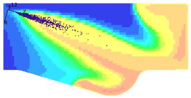
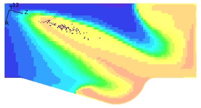
63 53 20CA Local max T= 2479K Local max T= 2472K 22CA Local max T= 2491K Local max T= 2476K 24CA Local max T= 2503K Local max T= 2476K 26CA Local max T= 2507K Local max T= 2468K 28CA Local max T= 2505K Local max T= 2459K 30CA Local max T= 2495K Local max T= 2454K

64 Cylinder Pressure [bar] 54 The combustion is visible since -2CA, as the local maximum temperature is suddenly increased. When comparing exact start of combustion, it should be taken in account, that the simulations are having different SOIs, as the table 5 shows in section 5.7. (The ECFM CLEH is starting the injection 0.3CAs later than ECFM 3Z.) The penetration of the spray is relatively same for both of the simulations, and the flame front is hitting the piston bowl at around 4CA. During the combustion propagation, it is visible that the ECFM CLEH has a little higher peak temperature. The most interesting thing is what happens in the center of the spray: There is a relatively cold, bowling pin shaped green area in the center of the spray. The temperature difference in that area is around 500K between the models, for example at 10CA. (This can be related to different modelling of the droplets evaporation, as ECFM CLEH takes into account the radial distribution of equivalence ratio around the droplets.) The flame is propagating and it reaches the liner at around 13-14CA as the piston moves down and lets the spray spread over the bowl. The dome is reached at 20CA by the flame. 6.2 Engine performance at 10% load At 10% engine load operation point, the ECFM 3Z combustion model was tested with two different ignition models, Standard and Double-Delay ignition models. The following Figure 29 shows the results of the auto-ignition model simulations Measurement Cylinder Pressure ECFM_3Z_1comp_stand Cylinder Pressure ECFM_3Z_1comp_dd Cylinder Pressure ECFM_3Z_5comp_dd Cylinder Pressure ECFM_3Z_5comp_stand Cylinder Pressure Crank Angle [ ] Figure 29. ECFM 3Z ignition models at 10% load As it is seen in Figure 29 above, the Double-Delay ignition model is completely poor with 1 component fuel implementation. Also the Standard ignition model with 5 component

65 Cylinder Pressure [bar] 55 fuel is relatively bad, as the pressure drops too low before the pressure rises due to combustion. The best match in maximum pressure and the cool flame phenomenon before the combustion pressure rise is reached with the Double-Delay ignition model with 5 component fuel. The second best is the Standard model with 1 component fuel. These are the two simulations that are chosen to be compared to ECFM CLEH simulations. Following Figure 30 shows the comparison between the combustion models through the whole simulation time domain Measurement Cylinder Pressure ECFM_3Z_1comp_stand Cylinder Pressure ECFM_3Z_5comp_dd Cylinder Pressure ECFM_CLEH_1comp Cylinder Pressure ECFM_CLEH_5comp Cylinder Pressure Crank Angle [ ] Figure 30. Cylinder pressure, 10% load The zoomed cylinder pressures at combustion stage are visible in adjacent Figure 31. The ECFM CLEH with 1 component fuel implementation shows similar behavior as the ECFM 3Z 5 component with Standard ignition model in Figure 29, the pressure drops too low before the combustion. Also the peak pressure is over predicted. In the figure the cool flame effect is visible at 2CA-3CA, where the ECFM 3Z with Double-Delay ignition model is capable to predict it nicely with 5 component fuel, but the start of combustion is still a little bit too early. The pressure rise and peak pressure are well modeled with ECFM 3Z Standard ignition model and ECFM CLEH 5 components fuel simulations.

66 Temperature [K] Cylinder Pressure [bar] Measurement Cylinder Pressure ECFM_3Z_1comp_stand Cylinder Pressure ECFM_3Z_5comp_dd Cylinder Pressure ECFM_CLEH_1comp Cylinder Pressure ECFM_CLEH_5comp Cylinder Pressure Crank Angle [ ] Figure 31. Combustion cylinder pressure, 10% load The averaged cylinder temperature is relatively well predicted with all the simulations. ECFM CLEH slightly over predicts the peak temperatures and also the expansion stage temperatures, as Figure 32 shows Measurement Cyl avg T ECFM_3Z_1comp_stand Cyl avg T ECFM_3Z_5comp_dd Cyl avg T ECFM_CLEH_1comp Cyl avg T ECFM_CLEH_5comp Cyl avg T Crank Angle [ ] Figure 32. Cylinder averaged temperature, 10% load Figure 33 shows the rate of heat release at 10% engine load. The maximum values of the heat releases are off from the measurement values, but the overall shape of the curve is

67 Momentary Heat Release [kj/deg] 57 more or less captured with all the simulations. The curves are slightly resembling the one in Figure 3, in Chapter 2. The ignition delay is relatively long, and there is some time for fuel to be mixed. (This is visible also in Appendix 4, where the λ=1 isosurface is already visible between -2CA and 4CA, indicating the mixed fuel zone. The local maximum temperatures are still low, reflecting that the combustion is not yet started.) At 10% load, the effect of short, premixed combustion is visible before the diffusion flame Measurement Momentary HR ECFM_3Z_1comp_stand Momentary HR ECFM_3Z_5comp_dd Momentary HR ECFM_CLEH_1comp Momentary HR ECFM_CLEH_5comp Momentary HR Crank Angle [ ] Figure 33. Rate of heat release, 10% load As it was discussed before, the ECFM CLEH 1 component simulation has delayed ignition compared to measurement. Also the bump of cool flame effect is nicely visible near 2CA by the ECFM 3Z Double-Delay with 5 component fuel, as discussed before. The ECFM CLEH with 5 component fuel has some similar effects visible: The start of combustion is exponentially growing, and the slope of heat release is not as steep as it is with Standard ignition model with ECFM 3Z.

68 Cumulative heat release [kj] Measurement Cum. HR ECFM_3Z_1comp_stand Cum. HR ECFM_3Z_5comp_dd Cum. HR ECFM_CLEH_1comp Cum. HR ECFM_CLEH_5comp Cum. HR Crank Angle [ ] Figure 34. Cumulative heat release, 10% load The curves for cumulative heat releases are illustrated in Figure 34. The best prediction of cumulative heat release is with the ECFM 3Z 1 component Standard ignition simulation, as the second best is ECFM CLEH 5 component simulation. The exact burnt fuel values, likewise the other performance values are visible in Table 10 below.

69 59 Table 10. Engine performance, 10% load Measurement ECFM 3Z ECFM CLEH Fuel implementation - 1 comp 5 comp 1 comp 5 comp Ignition model - Standard Double- Delay P_max [bar] P_max location from TDC [ ] BMEP [bar] T_max [K] 1,394 1,386 1,419 1,411 1,431 Cum. HR [kj] Error in Cum. HR [%] Cum. HR 50% location from TDC [ ] Heat release rate (max) [kj/deg] Start of combustion (10% from HR_max) [ ] TKI TKI Combustion duration [ ] The performance of the engine is relatively well predicted with ECFM 3Z 1 component Standard ignition and with ECFM CLEH 5 component simulation. Table 11 below shows the results for efficiency predictions of the 10% load simulations.

70 60 Table 11. Engine efficiency, 10% load Measurement ECFM 3Z ECFM CLEH Fuel implementation - 1comp 5comp 1comp 5comp Ignition model - Standard Simulated cycle piston work, -180CA to 140CA [J] Full cycle piston work, -360CA to 360CA [J] Double- Delay TKI TKI 4,281 4,425 4,185 4,530 4,510 4,382 4,526 4,286 4,631 4,611 Piston power [kw] Engine shaft power [kw] Fuel mass injected [g] Fuel LHV 41.3 MJ/kg [kw] Efficiency [%] Error in eff. [%] The predictions are not as desirable as for the 100% load case in tables 7 and 8. The engine efficiency is predicted with 1.71% error by ECFM 3Z Double-Delayed ignition 5 component fuel simulation, as the ECFM CLEH 5 component prediction has 9.54% error. The best match simulations are again chosen to evaluation with relative errors to measurement cylinder pressure. Figure 35 below shows the error curves for ECFM 3Z Double- Delay 5 component fuel and ECFM CLEH 5 component fuel simulations.

71 Pressure [bar] Error [%] Measurement ECFM_3Z_5comp_dd_pressure ECFM_CLEH_5comp_pressure ECFM_3Z_5comp_dd_error ECFM_CLEH_5comp_error Crank angle [ ] Figure 35. Cylinder pressure error, 10% load The effect of cool flame prediction is visible in error curves between 0CA and 5CA. The biggest error peaks are due to the early combustion of both simulations. Even though the slope of the pressure curves are right, the exact values are over predicted at 5CA to 10CA. This is the region where the fuel properties and auto-ignition coefficients are dominative. The ECFM CLEH has the potential to be much more accurate even in this pressure rise stage, if the ignition tables could be tuned. In these ECFM CLEH simulations the TKI tables are used, as they are implemented by Siemens. At the expansion stage after 35CA, the ECFM CLEH model performs again much better than the ECFM 3Z. The section view comparison is made also for the 10% load models in Table 12 below. It is again considered, that the start of injection is different due to the tuning of the models, as the values can be seen in the Table 6 at section 5.7. The ECFM CLEH model here has 1.2CA more delayed injection compared to ECFM 3Z simulation.

72 62 Table 12. Combustion section view comparison, 10% load ECFM 3Z Double-Delay 5 component ECFM CLEH 5 component -4CA Local max T= 897K Local max T= 898K -2CA Local max T= 899K Local max T= 901K 0CA, TDC Local max T= 905K Local max T= 900K 2CA Local max T= 972K Local max T= 897K 4CA Local max T= 2435K Local max T= 1074K

73 63 6CA Local max T= 2674K Local max T= 2201K 8CA Local max T= 2702K Local max T= 2458K 10CA Local max T= 2699K Local max T= 2437K 12CA Local max T= 2687K Local max T= 2482K 14CA Local max T= 2671K Local max T= 2483K 16CA Local max T= 2652K Local max T= 2479K 18CA Local max T= 2624K Local max T= 2448K

74 NOx [g/kwh] 64 It is illustrated in Table 12 above, that the combustion starts much later, even though the SOI is earlier than 100% load case. The injection duration is much shorter in this low load case. However, the penetration of the droplets is long and they are hitting the piston bowl before combustion. The rapid increase in local maximum temperature is indicating the start of combustion at 4CA. When the combustion is started, the flame propagation is really fast. The droplets have relatively long time period to evaporate and mix with air, so the air excess ratio is near one in many locations (This can be seen in Appendix 4, at 2-3CA, with 10% load isosurface and temperature comparison). At the beginning of the combustion, the flame propagation model is used more than the diffusion flame, as they both are modelled individually in the ECFM CLEH model. The liner is reached almost immediately as the mixture bursts into flame around 6CA. The flame propagates and touches the dome at 12CA. The local maximum temperatures are in general K higher in the ECFM 3Z combustion in this 10% load case, as it is visible also in the temperature contours. 6.3 NOx prediction Adjacent Figure 36 shows the results for the NOx predictions of all the models with different engine loads. The results have relatively high errors, but it was expected that the emission models are predicting relatively low emission rates %_load 100%_load Measurement ECFM 3Z 1comp ECFM 3Z 5comp ECFM CLEH 1comp ECFM CLEH 5comp Figure 36. NOx prediction of different simulations The 100% load cases had same order of magnitude results with both 3 Step Zeldovich and NORA emission models. The most accurate result was NOx rate of 11.14g/kWh (15.8% error) by NORA, ECFM CLEH with 5 component fuel, at 10% load engine operation point. The same model performed in 100% load point with result of 8.48 g/kwh

75 65 having error of 41.5%. The best 100% load prediction towards the emissions had the ECFM CLEH 1 component with result of 8.96g/kWh with error of 33.9%. It should be taken in account that the both emission models were not implemented with both combustion models, so the results are also affected by the varying combustion modelling. The emission modelling is more or less directional. Similar results can be found (Abouri;Zellat;Desoutter;& Cano, 2009), where the accuracy of the NOx prediction was around 20%. 6.4 Heat flux to walls Through many different studies in Wärtsilä, the ECFM 3Z has given relatively hot combustion results when it comes to heat transfer to walls. For example the heat flux to the piston is over predicted in many cases, and the surface temperatures are relatively high. (Wärtsilä) The comparison of the heat transfer capabilities were done for 100% load cases, because that is the most interesting engine operation point towards the heat stresses. The compared simulations in this section are both using 5 component fuel implementation. The results are cycle averaged through the simulation time domain for the sector model. The averaging range is -10CA +140CA. The results can be seen in Table 13 below. Table 13. Heat transfer comparison of sector models ECFM 3Z ECFM CLEH Difference [%] Engine load [%] MAX heat flux to the piston in hot spot [MW/m 2 ] Total heat to the dome [kw] Total heat to the liner [kw] Total heat to the piston [kw] Total heat to the walls [kw] The last column in Table 13 shows the difference in between the combustion models. The overall heat to the piston is almost 17% less in the ECFM CLEH model. That is relatively big number, when considering that the turbulence model and the wall treatment are exactly the same, as is the calculation mesh. The hot spot heat transfer has nearly 30% less heat in ECFM CLEH compared to ECFM 3Z due to the temperature differences in

76 66 the core of the combustion (as discussed in section 6.1, about the cold bowling pin effect in ECFM CLEH). Relatively big differences are illustrated in Figures 37 and 38. Figure 37. ECFM 3Z piston surface heat flux, W/m 2 It can be seen that the green area in the contour plots are similar in both cases. The scales are the same, so the pictures are comparable. Figure 38. ECFM CLEH piston surface heat flux, W/m 2 The measurements in different engines are showing same kinds of results, that the hot spot heat flux is more uniform, as it is here in ECFM CLEH model (Wärtsilä).

77 Fuel Film Mass [kg] Fuel film formation The fuel film formation is plotted only for 10% load simulations. At the 100% engine load, the film formation is negligible. Figure 39 shows the total fuel film mass on the walls during the 10% load simulations. 4.9E E E E-06 ECFM_3Z_10%_5comp_dd ECFM_3Z_10%_1comp_stand ECFM_CLEH_10%_5comp ECFM_CLEH_10%_1comp 2.1E E E E Crank Angle [ ] Figure 39. Fuel film mass, 10% load It is visible from the figure above that the 5 component models are having more fuel film than the 1 component ones. The fuel properties are different, and with 5 pseudo components fuel implementation, there are some particles with higher density. Those are the ones having high momentum and are most likely hitting the piston. The differences in the fuel spray penetration are illustrated in Table 14 below. The simulation cases in the table are both having the same SOI, so they are comparable in terms of spray penetration.

78 68 Table and 5 component fuel sprays, 10% load ECFM CLEH 1 component ECFM CLEH 5 component -4CA Local max T= 898K Local max T= 898K -2CA Local max T= 901K Local max T= 901K 0CA, TDC Local max T= 901K Local max T= 900K 2CA Local max T= 897K Local max T= 897K 4CA Local max T= 892K Local max T= 1074K Table 14 shows that the spray reaches the piston bowl around -2CA to 0CA, and there are much more droplets near the piston surface at 4CA. Those are the ones which can be transferred into the liquid film, as discussed in the section 4.5, if the circumstances are favorable. The total amount of film in the whole cylinder at 40CA after TDC is listed in Table 15. Also the percentage from the total injected fuel is calculated.

79 69 Table 15. Fuel film of the cylinder, 10% load ECFM 3Z ECFM CLEH Fuel implementation 1comp 5comp 1comp 5comp Ignition model Fuel film mass (at 40CA) [g] Fuel film mass (from injected fuel mass) [%] Standard Double- Delay TKI TKI 9.53E E E E The accuracy of the fuel film prediction is relatively hard to evaluate because no experimental data is available. It is easy to think that the fuel spray hits the piston, forming the film over the surface. After some time the film should decrease and little by little evaporate. This kind of phenomenon is captured in Figure 39, except the ECFM 3Z Double- Delay 5 component simulation. The film mass is increasing again at 5CA, and stays in the relatively high value. This kind of behavior has not been captured before, and it is not clear what is happening at this point. The film mass for liner and the dome are negligible also in this case, the shape of the curve is coming from the piston results. Table 15 shows that ECFM 3Z 5 component simulation with Double-Delay ignition model is creating 6.52% film from the injected fuel, which is a lot. As discussed before, the evaporation from the film is difficult. Practically the film stays as unburnt fuel. The film masses on the walls are plotted in 3D for every 5 components and are visible in Appendix 3. The mass fractions are visible in Figure 15 in section 4.6. As Appendix 3 shows, the component R5d is creating the most of the film mass, yet almost half of the injected fuel is modelled with the component in question.

80 70 7. CONCLUSIONS The two different combustion models, ECFM 3Z and ECFM CLEH, with different autoignition models, emission models and fuel implementations were tested in this thesis. The used reference engine is Wärtsilä 20, and the evaluation was completed for two engine operation points at 100% and 10% engine load. The geometry for in-cylinder model and the boundary and initial conditions were given. The calculation mesh study was made with mesh quality check. A lot of simulations were done with different models. The model parameters and coefficients were tested in order to match the measurements. The combustion models performance and capability to predict emissions rates and heat fluxes were determined. One of the most interesting thing of this thesis was to see the implementation of ECFM CLEH combustion model, and the newest version of the Star (v4.30) capability to predict the performance of medium speed engines diesel combustion. The results look promising. The ECFM 3Z combustion model has certain limitations regarding combustion modelling. It uses only one progress variable to model the flame propagation, as the ECFM CLEH uses one for auto-ignition and flame propagation, and one for diffusion flame. The models had different coefficients in order to match the measurements. As a more advanced model, ECFM CLEH has more logical and specified tuning coefficients. At 100% engine load, ECFM CLEH combustion model predicted the cylinder pressure curve with +/- 1.5% accuracy through the combustion time domain, as the ECFM 3Z had the accuracy of +/- 3.5%. Both models were able to predict 10% load pressure curve with accuracy of +/- 9.0%. In all the cases the exact maximum cylinder pressure was well predicted. Near the peak value of heat release rate, the ECFM 3Z had a little better accuracy, but the ECFM CLEH had more feasible results in the late combustion stage. The ECFM CLEH model was able to predict lower heat fluxes than the ECFM 3Z, which had relatively high heat transfer rates compared to Wärtsilä s experience. The 100% load case piston heat flux was nearly 17% lower in ECFM CLEH and the peak value as much as 30% lower in the hot spot on the piston surface. The IFO implementation was tested with 1 pseudo component approach as well as with 5 components approach. The fuel properties are highly related to auto-ignition and for example fuel film formation. At the 100% engine load the differences in cylinder pressure curves were relatively small, as expected. In some 10% load cases, for example, with Standard auto-ignition model the 1 component fuel had relatively good prediction of engine performance. Overall suggestion would be to use the 5 component fuel being more physical implementation of intermediate fuel oil, as it had better results in average. The fuel film formation was also highly affected by the fuel properties. Heaviest components had deeper penetration and slow evaporation rates.

81 71 The two different NOx models were tested alongside the combustion models. 3 Step Zeldovich with ECFM 3Z and NORA model with ECFM CLEH. Both of the models had relatively poor prediction for engine emission rates, the errors fluctuating from 13% to 51%. In the end, the NORA emission model had slightly better predictions, but the combustion was also modeled differently affecting to the NOx formation. Some uncertainties are here discussed, outside the turbulence and the combustion modelling, starting from the given geometry. In this thesis the narrow crevice between the piston crown and the cylinder liner was not modelled. The dome had unrealistically flat shape, and the small shape changes due to the pressure fluctuations were neglected. In the CFD calculations there were a lot of different coefficients and models, which needed to be set up correctly. Due to that the user mistakes were usual, and those were tried to squeeze down with usage of scripts. Some of the models that were used, but not validated in this thesis, had coefficients that can affect to combustion results. (For example in the spray model, there were coefficients that had values based on previous evaluation simulations done by Wärtsilä.) Even though, the IFO fuel is modelled in the simulations, the impurity of the real life fuel is a fact. The reference measurements and the boundary condition measurements are having the measurement errors and some of the initial conditions are already simulation results from another software. Also some physical things, that are not modelled, are having the impact to results. For example, the radiation heat transfer is not modelled as it is present in the real engine. Likewise the soot and other contaminants inside the cylinder and on the surfaces of the real engine parts are neglected, although the measurement engine is thought to be relatively clean during the measurements, shortly after assembly. Some suggestions for the future work are here provided. As being very sensitive towards the calculation mesh, the combustion modelling and heat transfer from gas to wall should be investigated with different meshes. With sector mesh, like used in this thesis, the incylinder velocity profiles should be captured more accurately near the wall to model the convective heat transfer correctly. Even though the computational cost would increase, at least one reference case could be calculated in more details, to have an idea of the heat transfer performance. Some, already in Star implemented sub-models could be worth of trying, for example different spray models. The most crucial investigations for future needs still to be done with the auto-ignition libraries (TKI tables) and the fuel properties. With tuned TKI tables the pressure curve fit should be done even more accurately with ECFM CLEH combustion model. For example at 10% engine load the pressure curve prediction error should be around +/-2%, as the biggest errors now are done due to the early combustion stage. Also the current fuel implementations should be corrected, as they are having some unphysical shapes in the saturation pressure curves, causing numerical errors during the simulations. One of the most interesting thing in the future would be to see the performance of ECFM CLEH combustion model in premixed, gas combustion and furthermore dual fuel engines.

82 72 8. REFERENCES Abouri, D., Zellat, M., Desoutter, G., & Cano, A. (2009). ADVANCES IN COMBUSTION MODELING IN STAR-CD: a new technique for automatic grid and mesh motion generation applied to Diesel combustion and Emission analysis. 19th International Multidimensional Engine User's Meeting at the SAE Congress. Detroit. Retrieved from Anttinen, T. (2005). Numerical Modelling of Combustion and Emission Formation in a Diesel Engine with Different Fuel Injection Characteristics. Master thesis. Bai, C., & Gosman, A. D. (1995). Development of methodology for spray impingement simulation. SAE Technical Paper Series Bai, C., & Gosman, A. D. (1996). Mathematical modeling of wall films formed by impinging sprays. SAE Technical Paper Series Berni, F., Cicalese, G., & Fontanesi, S. (2017). A modified thermal wall function for the estimation of gas-to-wall heat fluxes in CFD in-cylinder simulations of high performance spark-ignition engines. Applied Thermal Engineering, 115, pp Bracco, F. V. (1985). Modeling of engine sprays. SAE Technical Paper Series Chen, Y. S., & Kim, S. W. (1987). Computation of turbulent flows using an extended k-ε turbulence closure model. NASA CR Chen, Y., DeMauro, E. P., Wagner, J. L., Arienti, M., Guildenbecher, D. R., Farias, P. A., & Grasser, T. W. (2017). Aerodynamic Breakup and Secondary Drop Fromation for a Liquid Metal Column in a Shock-Induced Cross-Flow. Albuquerque: Sandia National Laboratories. Colin, O., & Benkenida, A. (2004). The 3-Zones Extended Coherent Flame Model (ECFM3Z) for Computing Premixed/Diffusion Combustion. Oil & Gas Science and Technology, 59, pp Retrieved from Colin, O., Jay, S., & Pires da Cruz, A. (2004). Detailed chemistry-based auto-ignition model including low temperature phenomena applied to 3-D engine calculations. Proceedings of the 30th Symposium of the Combustion Institute. Echekki, T., & Mastorakos, E. (2011). Turbulent Combustion Modeling. New York: Springer.

83 73 Glassman, I. (1996). Combustion (3rd ed.). London: Academic Press, Inc. Heywood, J. B. (1988). Internal Combustion Engine Fundamentals. New York: McGraw-Hill. International Energy Agency, statistics. (2018, 9 13). Retrieved from 20indicators&indicator=TPESbySource&mode=chart&categoryBrowse=false& datatable=balances&showdatatable=false International Maritime Organization. (2018, 9 13). Retrieved from Karvinen, R. (2012). Lämpötekniikan perusteet (EDE-02020). Termodynamiikka Osa I. Knop, V., Nicolle, A., & Colin, O. (2011). Modlisation des oxydes d'azote Extension du modle NORA aux voies autres que thermique. IFP Energies nouvelles Report L Launder, B. E., & Spalding, D. B. (1974). The numerical computation of turbulent flows. Comp. Meth. in Appl. Mech. and Eng., 3, pp Moukalled, F., Mangani, L., & Darwish, M. (2016). The Finite Volume Method in Computational Fluid Dynamics, An Advanced Introduction with OpenFOAM and Matlab. Switzerland: Springer International Publishing. Nieuwstadt, F. T., Boersma, B. J., & Westerweel, J. (2016). Turbulence, Introduction to Theory and Applications of the Turbulent Flows. Switzerland: Springer International Publishing. O Rourke, P. j. (1981). Collective Drop Effects on Vaporising Liquid Sprays. PhD Thesis, University of Princeton. Patankar, S. V. (1980). Numerical Heat Transfer and Fluid Flow. New York: Hemisphere Publishing Corporation. Reitz, R. D., & Diwakar, R. (1986). Effect of drop breakup on fuel sprays. SAE Technical Paper Series Siemens. (2018, January 26). STAR Methodology, For Internal Combustion Engine Applications Siemens. (2018, January 26). User guide for es-ice Sirignano, W. A. (1999). Fluid Dynamics and Transport of Droplets and Sprays. Cambridge University Press, New York.

84 74 Subramanian, G., Pires da cruz, A., Colin, O., & Vervisch, L. (2007). Modeling Engine Turbulent Auto-Ignition Using Tabulated Detailed Chemistry. SAE Technical Paper Taskinen, P. (2005). Modelling of Spray Combustion, Emission Formation and Heat Transfer in Medium Speed Diesel Engine. Doctoral thesis. Tennekes, H., & Lumley, J. L. (1972). A First Course in Turbulence (Vol. 15). Cambridge: The MIT Press. Torres, D. J., O'Rourke, P. J., & Amsden, A. A. (2003). Efficient multicomponent fuel algorithm. Combust. Theory Modelling, 7, p. 67. Wärtsilä. (n.d.). Technical report. Wärtsilä, market shares. (2018, 9 14). Retrieved from Weber, R. (2013). Combustion Fundamentals with Elements of Chemical Thermodynamics (4 ed.). Clausthal-Zellerfeld: Papierflieger Verlag. White, F. M. (1988). Fluid Mechanics (Vol. 2). Singapore: McGraw-Hill Book Compaby. Yanzhi, Z., Ming, J., Huiquan, D., Pengfei, W., Jiangxiang, W., Hong, L., & Mao-zhao, X. (2018). Numerical and experimental study of spray impingement and liquid film separation during the spray/wall interaction at expanding corners. International Journal of Multiphase Flow. Zellat, M., Abouri, D., & Duranti, S. (2007, April 15). Recent advances in diesel combustion modeling: The ECFM-CLEH combustion model: A new capability in STAR-CD. Detroit: 17th International Multidimensional Engine User's Meeting at the SAE Congress Retrieved from

85 75 9. APPENDIX 9.1 Appendix 1: Simulation initial and boundary conditions Running events BDC [deg] -180 TDC [deg] 0 Start of simulation [deg] -180 End of simulation [deg] 140 Fuel properties Used fuel, IFO C H32.38 Lower enthalpy [J/mol] Higher enthalpy [J/mol] Injector parameters Number of nozzle holes 8 spray angle [deg] 74 cone angle [deg] 8 ENGINE LOAD 100% 10% Cylinder initial conditions Air pressure at start (atm) [bar] Air temperature at start [K] Turbulent kinetic energy [ m^2/s^2] Turbulent dissipation rate [ m^2/s^2] Oxygen mass fraction Nitrogen mass fraction EGR mass fraction 0 0 Residual gases mass fraction 0 0 Cylinder boundary conditions Injection duration [deg] Piston temperature [K] Dome temperature [K] Liner temperature [K], Z -coordinate from the dome [mm] Z = Z = Z = Z = Z = Z = Z = Z = Z =

86 Appendix 2: Calculation meshes of the sector model 1. The old mesh done by Wärtsilä, at TDC 2. The replicated mesh, at TDC 3. The replicated mesh, at BDC

87 9.3 Appendix 3: Fuel film mass on walls for 5 different fuel components at 40CA, ECFM 3Z, 10% load 77

88 Appendix 4: ECFM 3Z 100% load and 10% load comparison with 5 component fuel and Double-Delay ignition model Fuel mixing isosurface λ=1 Temperature contour and spray droplets 100% load 10% load 100% load 10% load -5CA Local max T= 931K Local max T= 895K -4CA Local max T= 986K Local max T= 897K -3CA Local max T= 1756K Local max T= 897K -2CA Local max T= 2054K Local max T= 899K -1CA Local max T= 2145K Local max T= 901K 0CA, TDC Local max T= 2189K Local max T= 905K 1CA Local max T= 2212K Local max T= 931K

89 79 2CA Local max T= 2242K Local max T= 975K 3CA Local max T= 2256K Local max T= 1665K 4CA Local max T= 2291K Local max T= 2435K 5CA Local max T= 2306K Local max T= 2620K 6CA Local max T= 2312K Local max T= 2674K 7CA Local max T= 2330K Local max T= 2699K 8CA Local max T= 2366K Local max T= 2702K 9CA Local max T= 2400K Local max T= 2699K 10CA Local max T= 2397K Local max T= 2699K

90 80 11CA Local max T= 2435K Local max T= 2694K 12CA Local max T= 2462K Local max T= 2687K 13CA Local max T= 2477K Local max T= 2681K 14CA Local max T= 2482K Local max T= 2671K 15CA Local max T= 2488K Local max T= 2661K 16CA Local max T= 2476K Local max T= 2652K 17CA Local max T= 2469K Local max T= 2637K 18CA Local max T= 2471K Local max T= 2624K 19CA Local max T= 2475K Local max T= 2607K 20CA Local max T= 2479K Local max T= 2591K

91 81 21CA Local max T= 2486K Local max T= 2576K 22CA Local max T= 2491K Local max T= 2559K 23CA Local max T= 2498K Local max T= 2543K 24CA Local max T= 2503K Local max T= 2526K 25CA Local max T= 2506K Local max T= 2509K 26CA Local max T= 2507K Local max T= 2491K 27CA Local max T= 2507K Local max T= 2473K 28CA Local max T= 2505K Local max T= 2455K

92 82 29CA Local max T= 2502K Local max T= 2436K 30CA Local max T= 2495K Local max T= 2419K 9.5 Appendix 5: The Scouter 1. The screenshot from The Scouter 2. The code of The Scouter import numpy as np import matplotlib.pyplot as plt import matplotlib.animation as animation fig = plt.figure() ax1 = fig.add_subplot(2,2,1) # Pressure plot ax2 = fig.add_subplot(2,2,2) # Temperature plot