Master s thesis The Department of Geosciences and Geography Physical Geography

Transkriptio

1 Master s thesis The Department of Geosciences and Geography Physical Geography South American subduction zone processes: Visualizing the spatial relation of earthquakes and volcanism at the subduction zone Nelli Metiäinen May 2019 Thesis instructors: David Whipp Janne Soininen HELSINGIN YLIOPISTO MATEMAATTIS-LUONNONTIETEELLINEN TIEDEKUNTA GEOTIETEIDEN JA MAANTIETEEN LAITOS MAANTIEDE PL 64 (Gustaf Hällströmin katu 2) Helsingin yliopisto 0

2 Tiedekunta/Osasto Fakultet/Sektion Faculty Faculty of Science Tekijä Författare Author Nelli Metiäinen Laitos Institution Department The Department of Geosciences and Geography Työn nimi Arbetets titel Title South American subduction zone processes: Visualizing the spatial relation of earthquakes and volcanism at the subduction zone Oppiaine Läroämne Subject Physical Geography Työn laji Arbetets art Level Master s thesis Aika Datum Month and year May 2019 Sivumäärä Sidoantal Number of pages 82 + appencides Tiivistelmä Referat Abstract The South American subduction zone is the best example of an ocean-continent convergent plate margin. It is divided into segments that display different styles of subduction, varying from normal subduction to flat-slab subduction. This difference also effects the distribution of active volcanism. Visualizations are a fast way of transferring large amounts of information to an audience, often in an interest-provoking and easily understandable form. Sharing information as visualizations on the internet and on social media plays a significant role in the transfer of information in modern society. That is why in this study the focus is on producing visualizations of the South American subduction zone and the seismic events and volcanic activities occurring there. By examining the South American subduction zone it may be possible to get new insights about subduction zone processes. A particular point of interest is the relation of volcanoes and earthquakes to the trench, or in other words examining how far from the trench do they typically form or occur. To present this, a set of models, figures and animations were created using the Python programming language in Jupyter Notebooks. These notebooks utilize freely available software and aim to be easily understandable, reproducible and modifiable. For earthquakes, data from the United States Geological Survey (USGS) between January 1960 December 2017, and for volcanoes, data from the Smithsonian institution covering the Holocene were used. Three main visualizations were created: 1) an animation of all of the earthquakes occurring chronologically, where bar plots show their frequency according to every two degrees of latitudes, and their location and magnitude is shown on a map, 2) a cross-section view of the sinking slab s seismic structure on a selected latitude range, and 3) a static figure, which can portray several different aspects of earthquakes or volcanism, and their distribution on the South American margin using bar plots and a map. The visualizations show clearly the difference between segments of normal subduction compared to flat-slab subduction, especially in regard to volcanic activity or its absence. Visualizations also highlights the distribution of volcanoes and earthquakes, as across the margin volcanoes are present in areas where normal or transitional subduction is taking place and missing in flat-slab segments, and earthquakes occur at depths between km, and km distance from the trench. Deep earthquakes remain an important topic of interest, as little is known of them, and their study remains challenging. In many segments, seismic gaps, which are another topic of interest, are also present at depths between km. In conclusion, visualizations are an effective way of relaying large datasets in a way that is easy and fast to absorb, and make observation from. These models, figures and animations are useful especially due to their configurability, and can be shared to others to use in future works. Avainsanat Nyckelord Keywords South American subduction zone, earthquake, volcanism, subduction zone, flat-slab subduction, visualizations, model 1

3 Tiedekunta/Osasto Fakultet/Sektion- Faculty Matemaattis-Luonnontieteellinen tiedekunta Laitos Institution Department Geotieteiden ja maantieteen laitos Tekijä Författare Author Nelli Metiäinen Työn nimi Arbetets titel Title South American subduction zone processes: Visualizing the spatial relation of earthquakes and volcanism at the subduction zone Oppiaine Läroämne Subject Luonnonmaantiede Työn laji Arbetets art Level Pro gradu Aika Datum Month and year Toukokuu 2019 Sivumäärä Sidoantal Number of pages 82 + liitteet Tiivistelmä Referat Abstract Etelä-Amerikan alityöntövyöhyke on yksi parhaista esimerkeistä alityöntövyöhykkeistä, jossa merellinen ja mantereinen laatta liikkuvat toisiaan kohti. Lisäksi se on jakautunut useisiin lohkoihin, joissa alityöntövyöhyke käyttäytyy eri tavalla, erityisesti uppoavan laatan vajoamiskulman vaihdellessa normaalista matalaan. Tämä vaikuttaa vulkaaniseen toimintaan. Tiedon jakaminen on muuttumassa yhä visuaalisemmaksi, siksi tämä työ keskittyy Etelä- Amerikan alityöntövyöhykkeen, sekä siellä esiintyvien maanjäristysten ja vulkaanisten prosessien visualisoimiseen. Visualisoinnin avulla suurten tietomäärien välittäminen on nopeampaa, helpommin ymmärrettävää, ja usein myös kiinnostavampaa, kuin suurten tekstitiedostojen lukeminen. Tutkimalla Etelä-Amerikan alityöntövyöhykettä on mahdollista oivaltaa uusia asioita alityöntövyöhykkeistä. Eräs erityisen kiinnostuksen kohde on tulivuorten ja maanjäristysten suhde alityöntövyöhykkeeseen, toisin sanoen: kuinka kaukana, ja millä syvyydellä hautavajoamasta ne voivat esiintyä. Python ohjelmointikielellä luotiin helposti ymmärrettäviä, kopioitavia ja muunneltavia malleja, kuvia ja animaatioita Jupyter Notebook ohjelmistolla. Maanjäristyksiä varten käytettiin USGS:ltä saatavaa tiedostoa ajalta tammikuu 1960 joulukuu 2017, tulivuoritoimintaa varten Smithsonian laitokselta tiedostoa, joka kattaa Holoseenin. Kolme pääasiallista mallia luotiin: 1) animaatio kaikista maanjäristyksistä kronologisesti, jossa pylväsdiagrammit esittelevät niiden jakautumista joka toisella leveysasteella pylväsdiagrammin avulla ja niiden sijainti ja magnitudi näkyvät kartalla, 2) läpileikkauskuva alityöntövyöhykkeiden seismisestä rakenteesta tiettyjen leveyspiirien välillä, ja 3) staattinen kuva, jossa voidaan esitellä maanjäristysten tai tulivuoritoiminnan tiettyä erityispiirrettä ja sen jakautumista Etelä- Amerikassa kartan avulla, sekä pylväsdiagrammeilla. Visualisoinnit osoittavat selvästi eron normaalin ja matalan alityönnön välillä, erityisesti vulkaaniseen toimintaan liittyen. Ne myös osoittavat tulivuoritoiminnan ja järistysten jakaantumisen selkeästi, tulivuoritoiminnan keskittyessä normaalin ja siirtymävaiheisen alityönnön alueilla. Järistyksiä esiintyy km syvyydellä, ja km etäisyyksillä hautavajoamasta. Järistysten esiintyminen suurissa syvyyksissä on edelleen keskeinen tutkimuksen aihe, sillä syvistä järistyksistä tiedetään vain vähän ja tutkimus on hankalaa. Myös alueella esiintyvät seismiset tauot (seismic gap) km syvyydellä ovat tutkimusyhteisössä kiinnostava aihe. Visualisoinnit ovat tehokkaita suurten tietoaineistojen välittämisessä tavalla, jossa tieto on helposti ymmärrettävässä muodossa, ja havaintojen tekeminen on nopeaa. Tuotetut mallit sopivat hyvin jaettaviksi muulle tiedeyhteisölle ja kouluihin, erityisesti niiden helpon sovellettavuuden ja muokattavuuden vuoksi. Avainsanat Nyckelord Keywords Etelä-Amerikan alityöntövyöhyke, maanjäristys, tulivuoritoiminta, alityöntövyöhyke, visualisoinnit, mallinnus 2

4 TABLE OF CONTENTS ABSTRACT 1. INTRODUCTION LITERATURE & THEORETICAL BACKGROUND EARTH S STRUCTURE PLATE TECTONICS THE HISTORY OF THE PLATE TECTONIC THEORY THE IMPORTANCE OF TECTONIC PLATES SUBDUCTION ZONES FORCES DRIVING SUBDUCTION SUBDUCTION ZONE STRUCTURE SUBDUCTION ZONE LIFECYCLE FLAT-SLAB SUBDUCTION EARTHQUAKES AT SUBDUCTION ZONES THE MECHANICS OF SUBDUCTION ZONE EARTHQUAKES SHALLOW EARTHQUAKES INTERMEDIATE EARTHQUAKES DEEP EARTHQUAKES VOLCANISM AT SUBDUCTION ZONES VOLCANISM AT SUBDUCTION ZONES TYPES OF LAVA AT OCEANIC-CONTINENTAL SUBDUCTION ZONES VOLCANIC ROCK COMPOSITION TYPES FORMATION OF VOLCANOES SOUTH AMERICAN SUBDUCTION SOUTH AMERICAN FLAT-SLAB SUBDUCTION TRANSITION FROM FLAT-SLAB BACK TO NORMAL IN SOUTH AMERICA SOUTH AMERICAN SUBDUCTION ZONE SEGMENTS EARTHQUAKES IN SOUTH AMERICA VOLCANISM IN SOUTH AMERICA VOLCANIC ZONES IN SOUTH AMERICA ANDEAN MAGMAS METHODS DATA DATA PROCESSING WORKFLOW EARTHQUAKE VISUALIZATIONS VOLCANO VISUALIZATIONS RESULTS GENERAL OBSERVATIONS FROM ALL EARTHQUAKE DATA ANIMATION OF ALL EARTHQUAKES ALL EARTHQUAKES COMBINED ALL EARTHQUAKES BY MAGNITUDE CROSS-SECTION VIEWS

5 5.2 GENERAL OBSERVATIONS FROM ALL THE VOLCANO DATA ALL VOLCANIC STRUCTURE TYPES ALL VOLCANIC STRUCTURES ACCORDING TO ELEVATIONS ALL VOLCANOES VOLCANIC ROCK COMPOSITION TYPES PATTERNS AND CLUSTERING OF EARTHQUAKE DATA DEEPEST EARTHQUAKES STRONG TO GREAT MAGNITUDE EARTHQUAKES EARTHQUAKES BY DEPTHS INTERMEDIATE DEPTH EARTHQUAKES SEISMIC GAP GREAT EARTHQUAKES (M >8.0) DISCUSSION CHALLENGES ENCOUNTERED WHILE CREATING THE VISUALIZATIONS IMPLICATIONS OF THE EARTHQUAKE AND VOLCANISM VISUALIZATIONS ALL EARTHQUAKE VISUALIZATIONS AND VOLCANIC VISUALIZATIONS COMBINED CROSS-SECTION VIEW OF ALL EARTHQUAKES VOLCANIC ROCK COMPOSITION TYPES FUTURE VISUALIZATION DEVELOPMENT IDEAS CONCLUSIONS APPENDIX APPENDIX 1. JUPYTER NOTEBOOKS LINK APPENDIX 2: VISUALIZATIONS OF SOUTH AMERICAN SUBDUCTION ZONE EARTHQUAKES APPENDIX 3. VISUALIZATIONS OF SOUTH AMERICAN SUBDUCTION ZONE VOLCANISM BIBLIOGRAPHY

6 1. Introduction Subduction zones are complex dynamic systems interacting with the mantle and contributing to some of the most important geological processes on Earth, such as plate tectonics and the recycling of oceanic lithosphere (Stern & Gerya, 2017). They have an essential role in Earth s evolution and the development of continental crust (Van Hunen & Moyen, 2012; Zheng & Zhao, 2017). Through their significant role in the convection system, subduction zones have helped shape Earth into its present form and continue changing it (Van Hunen & Moyen, 2012). This thesis focuses on South American subduction zones and the processes related to subduction, such as volcanism and earthquakes. It is important to study more about the South American subduction zone, because it is unique in many ways. It is the world s longest continuous subduction zone (Hu et al., 2016; Stern, 2004), one of the only oceanic-continental convergent margins (Oncken et al., 2006), and its processes have led to the formation of the Andes, the world s longest mountain range (Schellart & Rawlinson, 2010). Subduction along the South American margin is also responsible for active volcanism and several magmatic processes occurring there (Oncken et al., 2006), as well as producing some of the world s deepest and strongest earthquakes (Stern, 2002). By examining the South American subduction zone, new insights about the processes and cycles operating there can be made, and our understanding of how subduction zones function can eventually lead to recognizing signs and patterns, which will help us predict earthquakes and volcanic eruptions and take action preventively to avoid casualties and economic damages. Expanding our understanding of the dynamic nature of Earth can also lead to new discoveries in geosciences, physics, chemistry, natural sciences and so on. In the current age of sharing information through the internet, and in particular, social media, visualizations play a significant role in the transfer of ideas and innovation. That is why in this study, the focus is on visualizing data into easily understandable and also easily replicated or modified models, figures and animations. Visualizations relay large amounts of information to people with just a glance, often in an interest provoking but comprehensible form. They can reveal things that are otherwise not as obvious, and can help in looking at situations or questions from a different perspective. Visualizations have a though-provoking component in them, which allows people to activate a creative side of their mind, and think outside of the box. This kind of thought processes can lead to groundbreaking ideas. A particular point of interest is the relation of volcanoes and earthquakes to the trench, or in other words examining how far from the trench do they typically form or occur and are there some noticeable differences here to other subduction zones, due to the unique characteristics of the South American subduction zone. Unlike many other subduction zones, the South American subduction zone consists of segments of normal and flat-slab subduction segments. Because of this the rate, angle, style and processes of subduction vary from segment to segment (Hu et al., 2016). 5

7 Overview of this study This study begins by briefly outlining the structure of Earth and how the different layers interact with each other. This is important to better understand plate tectonics and how subduction zones function, which will also be covered briefly. Furthermore, it has to be examined how subduction zones work in general, and what kind of processes they are involved in, before delving into South American subduction zones. In particular, the focus will be on earthquakes and volcanism, detailing mechanisms, functions and different theories. It is essential to understand how subduction zones typically function to appreciate how unique and complex subduction occurring in the South American oceanic-continental convergent margin is. After covering this general background information, the study continues into the South American subduction zone and the seismic and volcanic activity occurring there. The chapter will progress from one subduction zone segment to the next, describing each of their unique characteristics and behavior, focusing on volcanism and comparing normal and flat-slab subduction and seismicity at different depths along the subduction zone. The study will then progress into describing the methods used to make visualizations such as figures and animations of the South American subduction zone. A python script for producing models of South American subduction manifesting as earthquakes and volcanism was created especially for this study, and for future use for anyone to use freely for academic purposes. It is explained, how these models were made and how they could be utilized in future works. Some examples are shown and it is discussed, what kind of challenges were encountered and how they were dealt with. The models that were first mentioned in the methods are then examined in the results section, where the most significant points of interest are highlighted. These points will be revisited and analyzed in more detail in the discussion section, where some prominent theories will be presented to compare how well the models corroborate with previous studies. This way it is possible to assess both the models successfulness, but also whether the models support or challenge current theories. 6

8 2. Literature & theoretical background 2.1 Earth s structure In the past 50 years our knowledge of the structure and functioning of the surface and interior of Earth has significantly improved due to the development of technology and groundbreaking scientific research. According to our current understanding, Earth s interior structure consists of three main compositional layers: the core, the mantle and the crust. As Earth was forming, material began to differentiate according to density. The heaviest substances sank to form the core, while lighter substances rose to the surface (Van Der Pluijm & Marshak, 2004). Layers are also differentiated due to temperature differences, with the core being the hottest, and the crust being the coldest. It is unclear when the formation of a stable lithosphere and crust began. The core is at the center of Earth, at about 6370 km depth and extends to 2900 km depth, it has two layers; the solid inner core and the convecting outer core (Kearey et al., 2009). The core is hotter than the surrounding mantle, which heats up the core-mantle boundary and is the main heat engine behind mantle convection (Van der Pluijm & Marshak, 2004). The mantle can be divided into two sections. The lower mantle, also known as the mesosphere, extends from the core-mantle boundary at 2900 km depth to 670 km depth, while the upper mantle known as the asthenosphere comprises from about 670 km depth to the base of the more rigid lithosphere at roughly 100 km depth on average. A transition zone extending from km depth separates the lower and upper mantle (Kearey et al., 2009; Van Der Pluijm & Marshak, 2004). Together with the crust, the top layer of the mantle forms the lithosphere. Oceanic lithosphere typically has a thickness of about km, where the crust is about 7 10 km thick. Continental lithosphere on the other hand can reach a thickness of approximately km, with a typical crustal thickness of about 40 km (Kearey et al., 2009). The crustal thickness of continental crust can vary from 25 km at rifts, to > 70 km at young mountain ranges (Van Der Pluijm & Marshak, 2004). Oceanic and continental lithosphere differ from each other compositionally, structurally and in age. Oceanic lithosphere consists mostly of basalt, making it mafic in composition and structurally dense. It is formed at mid-ocean ridges, where asthenospheric mantle material forms new seafloor. As the lithosphere cools down, it becomes denser, slowly sinking as it ages. Because oceanic lithosphere begins sinking back into the mantle at a relatively early age, the structure of oceanic lithosphere is much less deformed and less complex than continental lithosphere. Indeed, due to its high silica content and felsic or intermediate composition, even though it is thicker, continental lithosphere has a less dense structure, making it relatively buoyant. Therefore, continental lithosphere resists subduction and can survive to be several billion years old, having gone through extensive deformation. Continental lithosphere is assumed to have formed through a complex cycle involving volcanic arcs, mountain building, erosion, sedimentation and reprocessing through the rock cycle (Van Der Pluijm & Marshak, 2004). The recycling of lithosphere is one of the most important processes on Earth, and affects mostly oceanic lithosphere (Stern & Gerya, 2017). 7

9 2.2 Plate tectonics Plate tectonics has become the basis for understanding several of Earth s processes, such as volcanism, earthquakes, orogeny and seafloor spreading The history of the plate tectonic theory There is undeniable evidence of the mobility of plates as well as the mantle, for example matching fossil and rock type findings, GPS measurements, and paleomagnetic measurements (Schubert et al., 2001). This has not always been the case. Scientists have long struggled to understand the dynamic nature of Earth and how it functions. In fact, due to the limited methods of studying the interior of Earth, many aspects still remain unclear. Even subduction zones and their processes are a relatively new discovery. The idea of the strong outer layer overlying the weaker asthenosphere was introduced in 1914 by Joseph Barrell. With it the concept of lithosphere was formed. Only later was it realized, that the lithosphere also functions as a thermal boundary layer as part of the convection system (Wessel & Müller, 2015). The plate tectonic theory is currently the most widely accepted theory explaining large scale processes in the solid Earth. It was developed from the continental drift theory, which was formulated by Alfred Wegener in Already in 1620 the first more detailed maps of the world were created, leading Francis Bacon to suggest that the East coast of South America and West coast of Africa fit together (Schubert et al., 2001). The continental drift theory was based heavily on the fact that the coasts of South America and Africa fit together, and was supported by geological evidence of related fossils, past climate zones, and matching rock formations on both continents (Stein & Wysession, 2003; Schubert et al., 2001). At the time of its creation, the theory was not able to explain how the continents could have feasibly drifted apart, and so the theory was largely dismissed, until around the 1960 s, when the first wide scale paleomagnetic measurements were made. These measurements provided evidence that the continents had been moving, based on the geometry and evolution of Earth s magnetic field (Stein & Wysession, 2003). In 1929 Arthur Holmes published his ideas about thermal convection driving continental motions, that form partly the base for Robert S. Dietz s and Harry H. Hess s suggestions of the seafloor spreading in 1961 and 1962 (Wessel & Müller, 2015). Hess mapped out the seafloor depth with echo-sounding surveys, and discovered mid-ocean ridges and trenches. Based on his discoveries, Hess proposed that new seafloor is being created at mid-ocean ridges, and being spread apart, and as Earth s surface area remains constant, is eventually subducted at trenches as it ages and cools down. Hess therefore came up with the first theory of seafloor recycling (Hough, 2004). The discovery of seafloor spreading inspired J. Tuzo Wilson, and in 1965 he proposed the essence of the plate tectonic theory. He came up with the idea of transform faults and is therefore sometimes credited with having created the idea of plates. He based the theory of the plates moving on the distribution of seismic activity along long mobile belts. Mobile belts contributed either to the creation, destruction or conservation of plates. These happened at mid-ocean ridges, trenches and transform faults respectively (Wessel & Müller, 2015). In 1967 Dan McKenzie and Bob Parker and in 1968 Jason Morgan both created the Euler pole theory, which modified the plate tectonic theory to work on the surface of a sphere (Bercovici et al., 2015). In 1969 after the plate tectonic theory had emerged, McKenzie hypothesized that both mid-ocean ridges and trenches were involved in the circulation of lithosphere, and in 1973 he and others published the 8

10 first models of mantle convection (Wessel & Müller, 2015). It is widely thought that the release of the mantle s gravitational potential energy through convective overturn drives plate tectonics. This all ties back to subduction zones, as they have a crucial role as part of mantle convection and the recycling of lithosphere (Bercovici et al., 2015) The importance of tectonic plates The plate tectonic theory is based on lithospheric plate movements. Seven major and several smaller lithospheric plates make up the surface of the Earth (Richards et al., 2000), though the number of major plates and minor plates varies according to different interpretation. These rigid plates move relative to each other over the weaker asthenosphere at a rate of a few centimeters per year. Plate motions are related to heat transfer and density differences (Moores & Twiss, 1995). Due to their rigidity, most deformation takes place at the plate boundaries, where it causes earthquakes, orogeny, volcanism and other tectonic phenomena (Stein & Wysession, 2003). According to the plate tectonic theory, there are three types of plate boundaries, where plates interact with each other. These are divergent boundaries, convergent boundaries and transform boundaries (Richards et al., 2000). At divergent boundaries, plates move away from each other and hot mantle material upwells at mid-ocean ridges. These act as spreading centers, where new oceanic lithosphere is being created. At convergent boundaries oceanic lithosphere descends back into the mantle at subduction zones. Convergent boundaries also include continental convergence, where two continental plates impact and deform, as at least one of the plates moves towards the other plate. At transform boundaries plate motion is parallel to the boundary, and plates slide against each other (Stein & Wysession, 2003). Plate boundaries are not always clear in areas where two or more large plates and one or more microplates interact. In these areas, broad deformation creates a plate-boundary zone where the geologic structure and therefore earthquake patterns are complex (Wessel & Müller, 2015). Due to the activity at plate margins, plates can grow, shrink or subduct completely, they can also be sutured together, or new plate boundaries can form when plates break up (Davies, 1999). In the plate tectonic theory, the lithosphere makes up the upper boundary layer of thermal convection in the mantle (Richards et al., 2000). The lithosphere is the cold, stronger outer boundary layer of the thermal convection system, which regulates Earth s cooling by transporting and releasing heat from Earth s interior (Stein & Wysession, 2003). This is enabled through heat transfer, the most important process on Earth (Beardsmore & Cull, 2001). Heat regulation is facilitated by two factors: hot and less dense material upwelling to the surface from the coremantle boundary due to its increased buoyancy, and cold lithosphere downwelling at subduction zones because of its increased density, sinking due to gravity. As the lithosphere is cold, it is also relatively strong, and therefore also a mechanical boundary layer. As well as physical differences, the lithosphere has a different chemical composition compared to the rest of the mantle, especially as the creation of crust in different settings and conditions allows for unique and distinct chemistry. This chemical variability is greatest in continental lithosphere. Therefore, the lithosphere is also a chemical boundary layer. Continental lithosphere is less dense, and therefore resists subduction because of its buoyancy, while oceanic lithosphere is denser and descends into the mantle as it cools down and sinks under its own weight. Due to the recycling of oceanic lithosphere between spreading ridges and subduction zones, no oceanic lithosphere aged 9

11 more than about 200 Ma exists. In comparison, continental lithosphere as old as several billions of years has been found (Stein & Wysession, 2003). It can therefore be said that plate tectonics explains the behavior of the lithosphere. It is the main surface manifestation of Earth s heat regulation, which in turn is responsible for the thermal, mechanical and chemical evolution of our planet (Stein & Wysession, 2003). Plate tectonics is a theory about Earth s horizontal surface motions, which has helped explain many tectonic processes witnessed on the surface (Richards et al., 2000). Plate tectonics is significant from the point it has enabled the creation of oceans and atmosphere through volcanism, hydrothermal circulation and the rock cycle. Plate tectonics also dictates climate to an extent, as the locations of large continents and mountain building affect both local and global weather conditions (Stein & Wysession, 2003). The plate tectonic mode of mantle circulation has likely enabled life on Earth. As new mantle material rises to the surface and old lithosphere sinks back into the mantle, plate tectonics drives the geologic carbon cycle through volcanism, erosion and weathering. The formation of mid-ocean ridges may have provided the necessary energy sources for the creation of chemosynthetic life (Bercovici et al., 2015). 10

12 2.3 Subduction zones Subduction has a significant, maybe leading role in plate tectonics. It is the primary engine of plate tectonics, as 90 % of the driving force is produced by the gravitational pull from the descending slabs (Van Hunen & Moyen, 2012). Subduction zones are also exceptional from the point that they enable the decoupling of plates at the surface. The creation and growth of continental crust is linked to subduction zone processes, and they also seem to be the only mechanism that allows the recycling of surface materials such as volatiles, sediments and water back into the mantle (Van Hunen & Moyen, 2012; Zheng & Zhao, 2017). Subduction zones are a central part of mantle convection, recycling raw material from the surface back to the mantle. These materials interact with the mantle, resulting in melting and the creation of magmas (Stern, 2002). Consequently, subduction zones have had a major role in influencing the compositional structure of Earth (Van Hunen & Moyen, 2012). Therefore, it can be concluded that subduction zones are surficial and interior expressions of Earth s prevailing tectonic mode, and they are also the dominant physical and chemical system of Earth s interior (Stern, 2002; Zheng & Zhao, 2017). Subduction may not, and likely has not always have been the way it is now. This is connected to the temperature of Earth s interior, which has undergone changes during Earth s evolution. Temperature controls the strength, density and composition of rocks, and so may have inhibited subduction earlier in Earth s history, or influenced the style of subduction or subduction processes. It is not yet clear when plate tectonics and subduction have begun on Earth (Van Hunen & Moyen, 2012). Subduction has an invaluable role in the convection system. Convection is the most important process in the mantle, as it determines the distribution of water and land, influencing the climate system and glaciation cycles, biological evolution and the formation of resources such as minerals and hydrocarbons. Convection is the main mechanism for heat transport from Earth s interior, and consequently plays a part in plate tectonics and the creation of continents, causing also earthquakes, volcanism and orogeny. Convection also influences the gravitational and magnetic fields (Schubert et al., 2001). In fact, subduction has played such an essential role in Earth s evolution, that it can be speculated whether continental crust would have developed without it, and if not, would terrestrial life have been possible. Their scale and role indicate that they are the most significant tectonic feature on Earth (Stern, 2002). Convergent margins can be divided into two kinds: subduction zones and collision zones. At subduction zones the sinking of an oceanic plate can happen under another oceanic or continental plate. At collision zones both plates are continental, or the other plate may be oceanic, but carries a magmatic arc. A subduction zone may also turn into an obduction zone or collision zone at the end of its existence, when the oceanic basin between the plates has been subducted. At this point the slab may detach from the surface plate (Schellart & Rawlinson, 2010). Presently, subduction zones reach a total length of km worldwide, and incipient subduction zones amount to km. Collision zones reach a total of km in length, meaning a total of km of plate boundaries are convergent plate boundaries ( 60,000 km for mid-ocean ridges) (Stern, 2002). Most of these boundaries are located at the edges of the Pacific Ocean, known as the Ring of Fire (Schellart & Rawlinson, 2010). 11

13 2.3.1 Forces driving subduction Heat from the core and mantle provides energy that drives convection, subduction and plate movements. These three are linked together and are interacting with each other, resulting in the dynamic nature of Earth. Earth s evolution into its current state is closely connected to them (Beardsmore & Cull, 2001). It is recognized, that heat provides the energy needed, but the question remains, what is the force that drives plate movements? It is argued that plate motion is in relative terms a passive phenomenon, as plate movements are caused by their gravitational potential energy (Van der Pluijm & Marshak, 2004). Gravity is a key factor driving large-scale motions on Earth. It acts on lateral density differences. Slabs are denser than the ambient mantle, which allows them to sink (Van Hunen & Moyen, 2012). Still, over the years there have been many different theories about what drives plate movements. Some arguing for the importance of basal shear traction, and some focusing on plate-boundary forces. The mantle drag theory alleges that plates move passively on a conveyor belt asthenosphere that drags them according to its movements, but it is likely the system is far more complex (Stein & Wysession, 2003). The edgeforce theory suggests that plates sink into the mantle under their own weight due to a density increase, and are then pulled into the mantle by forces acting on plate edges, such as slab pull (Grotzinger & Jordan, 2010; Fowler, 2014). Discrepancies with the mantle drag theory have made it unfavorable for Earth s current conditions, but there is evidence suggesting it may have been the primary driving force during the breakup of supercontinents (Kearey et al., 2009). Therefore, at the moment, the edge-force theory prevails. According to the edge-force theory, there are several forces affecting plates, such as slab pull, ridge push, trench suction and mantle drag. Slab pull is suggested to be its dominant force. Slab pull and ridge push are convective pressure gradients acting mostly on the edges of plates, while asthenospheric drag acts along the base of plates (Richards et al., 2000). Plate movement is triggered by two types of forces: driving and resisting forces (Fowler, 2014). Slab pull and ridge push are driving forces. They are manifestations of the thermal boundary layer (Davies, 1999). Both are caused by density differences in the mantle, and they are also linked to each other as hot mantle can only rise to the surface due to cold mantle sinking (Fowler, 2014). Slab pull The negative buoyancy of oceanic lithosphere is the main driving force for subduction and plate tectonics (Stern & Gerya, 2017). It is induced gravitationally (Stüwe, 2007), caused by the negative buoyancy of the descending oceanic lithosphere at trenches, and is proportional to the excess mass of the slab in relation to the mass of the mantle material it displaces (Wessel & Müller, 2015). Slab pull is a horizontal pressure gradient, created by a slab pulling away from the plate at the surface, leading to low pressure (Richards et al., 2000). Although it appears as if the slab is pulling the plate, in fact the plate feeds the slab into the mantle. Buoyant features resist subduction, but buoyancy is not strong enough to resist slab pull (Van Hunen &Moyen, 2012). 12

14 Trench suction Slab pull may cause small scale convection in the mantle wedge between the subducting slab and the upper plate. This convection can drag both the subducting plate and upper plate into the subduction zone, and is recognized as a force of its own: trench suction (Kearey et al., 2009). Trench suction may arise from the angle of subduction becoming steeper, causing the overriding plate to collapse towards the trench, or from roll back of the subducting plate, where the slab retreats from the overriding plate (Kearey et al., 2009). Ridge push (potential energy of the mid-ocean ridges) Ridge push was originally thought of as an edge force, meaning that it primarily acted at the edge of plates at the mid-ocean ridge, where the topographically high ridge s weight created the force as it slid down due to gravity, but now it is recognized ridge push has an effect across the area of the plate. It has been suggested that ridge push only affects lithosphere that is younger than 80 Ma old, because after reaching that age, it ceases cooling down significantly (Wessel & Müller, 2015). Ridge push may act as the only force driving plates, that lack descending slabs (Bercovici et al., 2015). Resistive forces Frictional forces between plates resist the forces that drive plate motions. They are linked to friction and buoyancy, and they hinder subduction. Resisting forces such as plate bending and mantle drag, which are caused by material deformation, together with phase change buoyancy effect, act as a counter balance for slab pull (Van Der Pluijm & Marshak, 2004). The main resistive forces such as mantle-drag and slab resistance occur as drag along the base of the plate and on the sinking slab (Fowler, 2014). Slab resistance acts primarily on the leading edge of the descending plate (Kearey et al., 2009). Basal drag can either increase or hinder motion. It is due to convection in the mantle, where the flow of asthenosphere creates drag at the base of plates. Plates move faster when the asthenosphere flows in the same direction as the plate is moving, and slow down when they move in different directions. It has even been suggested that if the flow of asthenosphere is at an angle to plate motion, it may change the direction of plate motion (Van Der Pluijm & Marshak, 2004). During subduction, the lithosphere s flexure is opposed by bending resistance. This force acts on the few tens of kilometers of the subducting plate at the surface close to the trench (Kearey et al., 2009). Another resisting force on subduction is the friction between the subducting and overriding plate. The overriding plate s resistance causes earthquakes at relatively shallow depths. The distribution of stress types may be determined by the balance between driving and resisting forces. If slab pull exceeds slab resistance and overriding plate resistance, the slab s subducting rate is faster and at shallow depths, the slab is thrown into tension. In the opposite situation, the slab is thrown into compression. The trench suction force acting on the overriding lithosphere causes it to be thrown into tension as well. The connectivity of a plate to a slab seems to strongly correlate with plate velocities, while size does not, meaning either there is a lack of mantle drag, or mantle drag is balanced out by distributed ridge push. These observations point to slab pull being the dominant plate driving force (Bercovici et al., 2015). Plates that do not have subducting 13

15 edges move at slower velocities, supporting the theory that slab pull is the main driving force (Fowler, 2014). At subduction zones the downgoing slab is both colder and denser than the mantle, causing a density contrast. Phase changes may strengthen the contrast of the slab in the mantle (Wessel & Müller, 2015). The phase transition of basalt into eclogite in the slab enhances sinking. This is because eclogite is dense and therefore cancels out the buoyancy of the lithosphere, causing the slab to become gravitationally unstable (Van Hunen & Moyen, 2012; Stern & Gerya, 2017). The phase transformation of basalt to eclogite takes place at the depth of ~40 km (Van Hunen & Moyen, 2012). Another phase transformation takes place once the slab reaches the olivine-spineltransition at 400 km depth (Kearey et al., 2009; Stüwe, 2007). Once olivine becomes spine, slab pull becomes stronger as the density of the slab increases. This phase change occurs in slabs earlier than in the surrounding mantle (Wessel & Müller, 2015). Metastable olivine wedges in slabs on the other hand can act as forces resisting subduction (Fowler, 2014). Last, the phase change of spinel and garnet to perovskite and magnesiowustite at km depth causes slabs to stagnate, and creates layered mantle convection, effectively pausing subduction (Van Hunen & Moyen, 2012). The transformation of garnet to perovskite releases water, which may cause the deepest earthquakes, at depth of over 500 km (Estabrook, 2003) Subduction zone structure Each subduction zone is different, but they display similar structural features (Moores & Twiss, 1995). Subduction zones vary according to trench and arc curvature, slab dip angle, bending curvature at the subduction hinge and at depth, according to the folding of slabs at and below the mantle transition zone, sub vertical slab edges, seismic gaps, slab kinks and slab tears (Schellart & Rawlinson, 2010). The structure of subduction zones may also change during their existence (Zheng & Zhao, 2017). They can be characterized by the structures of their thermal properties, as well as their geometric and geological properties. The structure of subduction zones may also change during their existence (Zheng & Zhao, 2017). The age of the seafloor reaching a trench is commonly ~100 Ma, with a thermal lithosphere thickness of ~100 km. Thickening and increasing density are related to age with oceanic lithosphere, and it becomes negatively buoyant in relation with the underlying asthenosphere at Ma. Therefore, at 100 Ma, the lithosphere sinks with ease, while subduction of seafloor under Ma resists sinking due to its buoyancy (Stern, 2002). The thermal structure of subduction zones is determined by several factors including the age of the subducting plate, rate of convergence of the plates and the geometry of subduction. These control the pressure-temperature conditions that drive metamorphic dehydration and partial melting at different depths. The thermal structure of subduction zones is also connected to the type of metamorphic fascies series in orogenic belts. The thermal structure may therefore control the temperature and fluid activity at the slab-mantle interface, which themselves affect the transport and ascent modes of crustal materials. Crustal rocks dehydrate more water in hotter conditions more rapidly than cooler ones, meaning that cold subduction zones are able to maintain more water to deeper depths. In hot subduction zones, much of the water is dehydrated 14

16 already in the forearc depths. Colder slabs also exhibit more arc magmatism and sub-arc earthquakes (Zheng & Zhao, 2017). Subduction zones can be divided into different kinds, depending on their characteristics. One of these categorizing methods is to divide subduction zones into Chilean or Mariana-type depending on how strongly the lower plate is coupled to the overriding one. Some subduction zones also exhibit double planes, or Wadati-Benioff zones, where two distinct planes are separated, and the upper plane experiences down dip compression, while the lower plane experiences down dip extension (Schellart & Rawlinson, 2010). Subduction is a process where two plates converge, but the nature of the subduction zone s plate interface can be to migrate backwards (trench/hinge or slab retreat, rollback, retrograde slab motion) or forward (trench/hinge or slab advance) over time. A significant majority of subduction zones migrate backwards. Factors controlling trench kinematics are the boundary conditions at the trailing edge of the descending plate, slab width, and the strength of the slab relative to the ambient upper mantle (Schellart & Rawlinson, 2010). The dip between the converging plates defines the geometric structure of subduction zones (Zheng & Zhao, 2017). Old plates sink at a steep dip angle (> 40) but with slower rate, causing trench roll back, which means the trench moves towards the ocean. Younger plates resist subduction and therefore have shallower dip angles (< 30), but also have generally higher rates of subduction. The angle of the dip is linked to the rate of slab subduction and the age of the slab. The slab dip angle may change during the existence of the subduction zone, and some subduction zones exhibit shallow subduction from forearc depths to subarc depths, deepening at postarc depths over 200 km (Zheng & Zhao, 2017). The dip angle controls the flow of the asthenosphere in the mantle wedge, with shallow dip angles inhibiting flow. Shallow dips also influence the strength of coupling between the plates; plates with strong coupling experience higher magnitude earthquakes. Subduction zones where plate coupling is weak commonly have active back arc basins (Stern, 2002). Trench The trench is a steep valley, where the two lithospheric plates meet, and the oceanic lithosphere bends in order to sink into the mantle. The trench is preceded by an outer swell, which is a topographic high, usually a few hundred meters higher than the surrounding abyssal plain (Fig. 1). The outer swell is likely the result of bending, and usually exhibits faults. Trenches tend to be about 5 10 km deeper than the surrounding ocean floor (Moores & Twiss, 1995). The age of the oceanic lithosphere influences the depth of the trench (Stern, 2002). Arc-trench complex Mature subduction zones create arc complexes in the overlying plate s lithosphere. A widely accepted theory suggests that arcs represent the initial stage of continental crust development, and hold a key role in the growth of continents. Depending on their location, arc complexes have very different characteristics, including structure, thickness and processes. Arcs formed on continental lithosphere (Andean-type) are very thick, up to 80 km, meaning they are twice as thick as normal continental crust. Here thickening is due to shortening and possible magmatic underplating. Arcs formed on oceanic lithosphere (intraoceanic or primitive) are much thinner, at 15

17 20 35 km. Arch-trench systems have three key portions, which have different structures and where different processes occur. They are the forearc, magmatic arc and back arc (Stern, 2002). Figure 1. Subduction zone structure. The subduction zone has several distinctive parts, that all have unique behavior and processes occurring. This is a representation of normal subduction with associated volcanism (Stern, 2002). Forearc Forearcs are typically located between the trench and the magmatic front (magmatic arc), and reach widths of km (Stern, 2002; Moores & Twiss, 1995). Forearcs may be accretionary or non-accretionary, meaning that they either grow through the addition of sediments or do not. Around half of convergent margins are accretionary, which is determined by the thickness of the subducted sediment (Stern, 2002). As accretionary forearcs need a significant supply of sediments, they develop close to continents (Moores & Twiss, 1995). Sediments as thick as m are prone to being scraped off and transfer to the overriding plate, although as much as 80% of subducted sediments are not accreted. The sediments that are added by frontal accretion form the accretionary prism or wedge. Sediments can also be added through underplating in the subduction channel. The accretionary prism consists of significantly deformed sediments, which dip towards the arc and undergo thrusting. Sediment emplacement age becomes older closer to the arc. Forearc basins form between the prism and magmatic arc (Stern, 2002). In subduction zones deformation of the crust begins at the base of the inner trench wall and focuses on the 16

18 accretionary prism. Thrust faults and strike-slip faults are common in accretionary prisms (Moores & Twiss, 1995). In areas where sediment supply is insufficient, non-accretionary forearcs develop. They usually have inadequately developed forearc basins, or lack them entirely. Instead, their igneous structure is exposed. Non-accretionary forearcs are not shielded by the accretionary prism, but are susceptible to subduction erosion, which can take the form of basal erosion or frontal erosion. Frontal erosion occurs typically when seamounts are subducted, disrupting the topography of the base of the inner trench wall. Basal erosion on the other hand causes scraping of the base of the upper plate by the rough seafloor. This scraping or rasping is enhanced by the horst-and-graben faulting that is created by the bending of the plate, between the forearc bulge and the trench (Stern, 2002). Forearc formation is connected to extension at the initial stages of subduction. Forearc crust is therefore likely formed by seafloor spreading. Ophiolites, or oceanic material trapped inside continental lithosphere are commonly parts of forearc basements. They become trapped and emplaced in continental lithosphere during the termination of subduction zones and consequent beginning of continental collision (Stern, 2002). Magmatic arc As referred to in their name, magmatic arcs are tectonic settings where melted mantle rises to the surface (Fig. 1). They can be described as linear arrays of point source loci volcanism, due to mantle wedge Rayleigh-Taylor instabilities. In comparison, mid-ocean ridges are line source loci, and hot spots are point source loci of volcanism, caused by upwelling and decompression melting for the former and intrinsic melt inducing processes in the deep mantle for the latter. Compared to the other two magmatic tectonic settings, arcs stay relatively fixed in relation to the melt zone in the asthenosphere. This allows the crust to thicken significantly, which consequently affects the ascending magma and its processes (Stern, 2002). Magmatic arcs are generated as a result of the significant decrease of athenospheric mantle melting temperature, which is due to the release of hydrous fluids from the slab. The lowered mantle melting temperature allows a zone of melt to form in the overlying asthenospheric mantle, to supply arc volcanoes with magma. Heat flow is high in the magmatic arc and back arc region, unlike in the forearc region. In fact, the magmatic arc signifies the beginning of the magmatic front. It is located km above the inclined seismic zone, and is likely related to the depth at which the slab reaches a sufficient temperature for melting. Most of the igneous activity takes place closest to the magmatic front and fades out as the distance from the trench increases. The spacing of arc volcanoes does not seem to follow a pattern, but is likely controlled by the thickness of the overriding plate s lithosphere, melt source gravitational instabilities or the distance between hot fingers that rise into the mantle wedge (Stern, 2002). 17

19 Back arc region Behind the arc, the back arc region may be in extension or compression resulting in thrusting and folding, depending on their strain class. Low strain arcs exhibit active extension and behave similarly to mid-ocean ridges. Here rifting and seafloor spreading take place at rates of ~16 cm/a for fast extension, to 4 cm/a for slow extension. Corresponding to the rate of spreading, the ridge morphologies, magmatic activities and features vary. Inflated ridges with axial magma chambers are caused by fast spreading, and axial rifts with portions of exposed mantle and lower crustal sections are caused by slow spreading. Rifted back arc basins can also be amagmatic, i.e. do not produce magma. High-strain convergent margins exhibit back arc regions experiencing crustal shortening and compression. The ensuing system of retroarc forland basins are commonly associated with the subduction of young, buoyant lithosphere, such as is the case with the Andean system, which is still active. Convergent margins with active back arc basins are associated with weak coupling, and therefore weaker earthquakes. If the slab is old and cold, then coupling is even weaker (Stern, 2002). 18

20 2.3.3 Subduction zone lifecycle Initiation and cessation The formation of a subduction zone requires the buildup of stress in the lithosphere over time. The lithosphere is relatively strong, and requires large amounts of stress to break, especially cohesive oceanic lithosphere ruptures only under immense tension. Therefore subduction zones typically form in areas of prior weakness. In the case of oceanic lithosphere, subduction initiation mostly occurs in areas where faults already exist (Stern, 2004). When subduction zone initiation occurs in continental areas, suture zones, where two plates have collided and merged previously provide suitable conditions for easier rupture (Condie, 1997). The mechanisms that trigger subduction zone formation are not yet clear. It has been suggested subduction initiation may occur in two ways: spontaneously or through induced nucleation. Spontaneous initiation happens, when the oceanic lithosphere collapses under its own weight and begins to sink into the mantle. The theory of spontaneous initiation is still insufficient in explaining how the beginning stages of sinking progress into actual subduction. Induced nucleation is more complex, and several different factors have been suggested to lead to it (Stern, 2004). One theory proposes that the failed attempt of subducting oceanic lithosphere in another subduction zone would cause tension to gather in both the subducting and overriding plate, until the lithosphere gives in in a zone of weakness, such as in fault or fracture zones (Condie, 1997). Another possibility is that the collision of continental plates causes the lithosphere to rupture far away from collision zones, in zones of weakness, due to stress transfer. Yet another theory suggests that polarity reversals in subduction zones may cause the initiation of new subduction zones, as the roles of the subducting and overriding plate are reversed and the direction of subduction changes. All of these theories, simplified, propose that plate movements cause tension, which ultimately leads to the rupturing of the lithosphere and the formation of a new subduction zone (Stern, 2004). Subduction zones may experience failure when strongly buoyant material enters the trench disrupting downwelling (Stern, 2002). Subduction zones may also cease to function during episodes of lowered or increased mantle temperature conditions. When the temperature is lower, adiabatic decompression melting decreases, causing ridge lock at mid-ocean ridges and affecting subduction. Increased temperature speeds up the production of new oceanic lithosphere at midocean ridges, and causes the oceanic lithosphere to be significantly thicker. Due to its thickness, the cooling of the oceanic lithosphere is slower, and because of its strong buoyancy, it fails to sink into the mantle leading to trench lock (Stern, 2004). Subduction ends naturally, once the oceanic portion of the sinking lithospheric plate has been subducted, and the collision of continental lithosphere begins (Stern, 2004). 19

21 Fate of subduction during/after continental collision The dynamics of the convergent system change significantly, when a subduction zone encounters and interacts with continental lithosphere and continental lithosphere enters the subduction zone. Subduction eventually changes into continental collision, which is a complex process due to continents differences in formation, composition, age and thermal history. The strength of the continental lithosphere is determined for example by its mineralogical composition and structure, thermal history, fluid content, grain size and pore fluid pressure. The end results of continental collision are influenced by several factors such as plate convergence rate, the composition and thermal structure of the continental lithosphere and the strength of the continental lithosphere (Magni et al., 2013). What happens when subduction turns into continental collision has been studied vastly, but remains uncertain. Numerical models have suggested there are three ways slabs may behave: detach, delaminate or behave in a manner that is somewhere between these two. Detachment of the slab happens when the crust and lithospheric mantle are strongly coupled, leading to subduction slowing down and the slab eventually breaking. Elevated lower crustal viscosity and interaction between the continental and oceanic portions of the slab lead to the oceanic portion eventually undergoing necking and breaking off. This is enabled through high tensile stresses and thermal weakening. Meanwhile, the continental portion continues collision, which due to high lower mantle viscosity leads to trench advance until break-off of the slab takes place (Magni et al., 2013). Oceanic subduction zones produce accretionary orogens while continental subduction zones produce collisional orogens, when continental lithosphere collides with another continental plate or marginal arc terrane. Continental subduction zones may lose their orogenic roots through slab breakoff and lower crust delamination or foundering (Zheng & Zhao, 2017). Delamination is likelier to happen with lower low mantle viscosity and low convergence velocity. In delamination, the upper crust and mantle lithosphere separate, and subduction of the slab continues, only now it consists solely of the mantle lithosphere. Trench roll back continues with delamination, as the delamination front moves further away from the initial suture zone. In an intermediate mode, the crust and mantle lithosphere are partially coupled, and the buoyancy of the continental crust inhibits subduction, causing it to slow down until the oceanic portion of the slab detaches from the continental lithosphere. Although the delamination front first moves away from the suture zone, it later becomes stationary (Magni et al., 2013). Fate of slabs after sinking Slabs may stagnate and pond at the 660 km transition zone, or penetrate into the lower mantle (Van Hunen & Moyen, 2012; Stern, 2002; Lundgren & Giardini, 1992), depending on their strength and buoyancy, also trench rollback may influence the slabs behavior (Van Hunen & Moyen, 2012; Agrusta et al., 2017). Other factors causing stagnation are the old age of slabs, decreased upper plare forcing and the arrival of another, more hydrated slab (Agrusta et al., 2017). Tomographic studies imply that slabs that do not penetrate into the lower mantle are lying above the 670 km seismic discontinuity (Lundgren & Giardini, 1992). It appears that most slabs penetrate into the lower mantle, there doesn t seem to be any correlation between the young age of the subducting plate at the trench and the slabs ability to sink into the lower mantle. This is most likely due to the long time it takes for slabs to reach the core-mantle boundary. Even a relatively fast sinking slab, 20

22 for example 10 cm yr-1 would take 29 Ma to reach the lower core-mantle boundary (Stern, 2002). Cold slabs are more likely to stagnate at the mantle transition zone, while young hot slabs (about 25 Ma) sink into the lower mantle (Agrusta et al., 2017). Stagnation may occur when the endothermic phase transition of the dominant mantle minerals turns spinel to perovskite, making the slab more buoyant relative to the mantle and increasing the mantle s viscosity. Because the lower mantle has a high density basaltic composition, it may form a barrier that inhibits slab penetration deeper into the mantle (Van Hunen & Moyen, 2012) Flat-slab subduction Globally, almost 10 % of active subduction zones exhibit flat-slab subduction. It is also likely other subduction zones have previously experienced flat-slab subduction. This would explain patterns of deformation and plate magmatism on their overriding plates (Bishop et al., 2017). It has been suggested that flat-slab subduction has had an important role regarding continental growth (Van Hunen et al., 2004). Flat-slab subduction occurs, when the initially normally dipping slab reaches the depth of about km, and dips at a nearly horizontal angle before becoming steeper again (Bishop et al., 2017). What causes flat-slab subduction is not entirely clear. Many different theories exist, and it seems that some key factors leading to it may include the relatively young the age of the subducting slab (<35 Ma), advancing overriding plate motions and buoyant features of the descending plate such as aseismic ridges or oceanic plateaus (Van Hunen & Moyen, 2012, Manea et al., 2017). Aseismic ridges decrease the density of oceanic lithosphere, making it more buoyant, they are also thicker than oceanic crust, thus do not deform or bend as readily as normal oceanic crust. It has also been suggested that regions of low-viscosity in the mantle wedge could promote slab flattening through reduced viscous resistance. This is due to changes in the viscosity and geometry of the mantle wedge (Bishop et al., 2017). In theory, a thicker, cooler mantle holds the subducting plate stationary, while the overriding plate moves on top of it. Another theory claims that the overriding plate advancing faster than the slab subducts can lead to flat-slab subduction. The overriding continental plate may also cause flat-slab subduction if it has a thick continental root, which couples the subducting slab to the overriding plate due to hydrodynamic suction force. It seems probable that flat-slab subduction lasts long after buoyant features have been subducted. This could explain what caused some now extant flat-slab regions, although no buoyant features are visible anymore (Hu et al., 2016). Also slab suction may have some influence slab flattening (Bishop et al., 2017). Slab suction is thought to create a low-pressure wedge into which the slab is pulled, as the slab drags down mantle material when it sinks (Van Hunen & Moyen, 2012). Another theory suggests that flat-slab subduction may be caused by an increase in the nonhydrostatic pressure forces, which are associated with subduction driven flow within the asthenospheric wedge. The suction force prevents the slab from sinking further into the mantle, and increases with the velocity of subduction, the viscosity and the narrowness of the mantle wedge (Manea et al., 2012). The transition from normal subduction to flat-slab subduction is associated with several events, such as the migration and spreading of the volcanic front arc magmatism, uplift and deformation, broken foreland and basement uplift, as well as basin subsidence. The migration of the volcanic front and expansion of arc magmatism are often associated with the beginning stages of a slab 21

23 flattening. The migration coincides with the decrease of magma and the decline of dehydration in the slab. The slab flattening may also result in broken foreland, due to thermal weakening of the crust the faulting that follows (Ramos & Folguera, 2018). Established flat-slab subduction on the other hand is often characterized by a lack of volcanism (Stern, 2005). Volcanism fades out as the slab flattens and moves horizontally under the overriding plate. As the slab is not at a depth where melts are created, nor is there any intervening wedge of mantle material between the plates, partial melting is inhibited; no magma is being created for the volcanoes, and they become extinct or are not able to form. No arcs therefore develop after flatslab subduction is established. Volcanism may resume later in areas where the slab reaches the depth of melting, and partial melting in the mantle wedge is enabled once more (Gutscher et al., 1999). 22

24 2.4 Earthquakes at subduction zones Subduction zones produce 80 % of all the seismic events on Earth, including the strongest and deepest earthquakes (Fowler, 2014). Subduction zones are highly active, dynamic systems, where the interaction between the plates and between the plates and the mantle causes frequent earthquakes and drives many other processes (Scholz, 2002). Subduction zones are capable of producing the strongest magnitude earthquakes. The largest earthquakes usually take place in areas where the subducting plate is only several tens of millions of years old. Young plates are relatively young and hot, and the rate of subduction is high (Satake & Atwater, 2007). Due to their high temperature, they are also relatively buoyant and therefore mostly shallow-dipping. This is a suitable setting for thrust faulting (Stein & Wysession., 2003). All of the earthquakes that have been M 9 or above, recorded in written history, have occurred at subduction zones that are under 80 million years old and converging at rates between mm each year (Satake & Atwater, 2007). At subduction zones, strongly coupled plates experience higher magnitude earthquakes. Coupling Is related to the age and dip angle of plates subducting. Therefore younger, shallowly subducting plates exhibit the highest magnitude earthquakes. Very shallow earthquakes (<50 km) are associated with coupling between the subducting and overriding plate. At this depth range, weakly coupled plates, which correlate with older age of the lithosphere, exhibit smaller magnitude earthquakes than strongly coupled plates (Stern, 2002). Large magnitude earthquakes often recur in areas they have struck at before. Earthquake records seem to point to large magnitude earthquakes occurring at relatively regular intervals. The time spans of these intervals vary, but mostly large earthquakes do not recur in short time spans, as it takes time to build up enough strain (Ohnaka, 2013). Large magnitude earthquakes are the most devastating, and they are sometimes preceded by smaller foreshocks, and almost always followed by aftershocks (Hough, 2004). Aftershocks release remaining local strain, as the bedrock adjusts and settles (Fowler, 2014). Earthquakes in subduction zones occur at much greater depths than anywhere else on Earth. In most areas that experience earthquakes, seismicity is limited to the surface, usually up to 20 km (Stern, 2002). Subducting slabs can be observed through seismic events deeper in the mantle. This is because subducting slabs are colder and stronger than the surrounding mantle, which is represented in the travel times of seismic waves. Deep earthquakes occur in these inclined zones of seismicity also known as Wadati-Benioff zones (Stein & Wysession, 2003). Changing tectonic environments cause subduction zones to exhibit several types of earthquakes at different depths and due to different focal mechanisms (Stein & Wysession, 2003). Seismic events take place mostly at the boundaries of plates, but also some intraplate earthquakes have been interpreted as representing old subduction zones in areas where converging of plates is still happening (Kanamori, 1986). Depending on the local bedrock, the fault s structure and earlier rupture history, each earthquake is a unique event (Hough, 2002). Subduction zone earthquakes are uniquely influenced by the sediment and water involved in the subduction process and changes happening to the ascending plate. Because of this, there is a much bigger range of earthquake types and processes (Scholz, 2002). Although subduction zones are seismically very active, parts of subduction zones exhibit so called seismic gaps. Here seismic activity is lacking, but seismic gaps also represent areas where future 23

25 earthquakes may strike, as it is theorized that during pauses in seismicity, these segments are gathering tension which will eventually lead to earthquakes. The frequency of seismic events is connected to the subduction zone s bathymetric or geological characteristics (Fowler 2014). The rate of subduction has an effect on earthquakes, as fast subduction of young lithosphere seems to produce more earthquakes than the slow subduction of old lithosphere (Stern, 2002). Closer to the surface the weight of the slab causes extension, while deeper it meets resistance from stronger mantle material and experiences compression (Stein & Wysession, 2003). The strain regime in the overriding plate is also related to the age of the sinking lithosphere, and the absolute motion of the overriding plate. Chilean type subduction zones are strongly coupled and experience strong compressional strain (Stern, 2002). The seismogenic zone in subduction zones is typically located between km depth. Above this depth, rocks and sediments along the interface are weak, and therefore mostly aseismic. The updip limit is speculated to be controlled by either the increasing strength of materials, the position of the subduction channel control point, pore pressure change or dehydration and alteration of smectite clays. The downdip limit controls the landward extent of the seismic zone and is connected to the depth of the Moho. Its location is likely controlled by the weakness of rocks, due to either too hot temperatures ( 350 C), or serpentinization, which makes rocks inherently weak. In the subduction of young, hot slabs, the Moho and downdip limit may appear at relatively shallow depths, as the temperature is higher closer to the surface. For old and cold subducting slabs, reaching 350 C temperatures lies much deeper in the mantle, and so the seismic zone extends deeper (Stern, 2002). The link between the seismogenic zone and Moho depth imply that the mantle beneath the forearc is most likely weak. This is due to the release of fluids from the slab and subsequent serpentinization. Continental forearcs are assumed to be stronger, due to their thicker crust, which may partially explain why many of the strongest earthquakes take place at oceaniccontinental subduction zones. Some convergent margins exhibit double seismic zones, where the other, lower seismogenic zone is located inside of the slab. Here the updip limit is controlled by the waning of serpentinite and the downdip limit is determined by the 350 C isotherm in dry peridotite. It has been suggested that earthquakes deeper than 50 km are related to the thermal state of the subducted lithosphere, and maximum depth would reflect how long it takes for the subducted slab to heat up to a point where rupturing is no longer possible. Therefore, earthquakes occurring in great depths are interpreted to indicate the slab is still relatively cool compared to the surrounding mantle. Slabs are heated by conduction, so it is reasonable to assume that the older, and therefore colder and quicker sinking slabs would have the strongest influence to depress geotherms, heat up slowly and exhibit the deepest earthquakes (Stern, 2002). 24

26 2.4.1 The mechanics of subduction zone earthquakes Most earthquakes occurring in the crust are caused by the build-up and release of strain. The movement and interaction of lithospheric plates creates strain, and earthquakes are the result of long-term strain in the bedrock being released when rock breaks and the plates jolt into their new positions (Shearer, 1999). All three main fault types can be found in subduction zone environments, and typically faults display a mixture of fault types (Stein & Wysession, 2003). These are: normal faults, reverse faults and strike-slip faults. Normal faults are extensional and present themselves as the downward movement of the hanging wall. Reverse faults include thrust and overthrust faults. Reverse faults are compressional and cause the upward movement of the hanging wall. When the dip angle of faults is less than 45, they are classified as thrust faults, when the angle is more than 45, they are overthrust faults. Both normal faults and reverse faults are so called dip-slip faults, where movement is vertical, while strike-slip faults, which are the third type, cause horizontal movement between fault surfaces (Shearer, 1999). Subduction zones have unique structures, which influence the seismic behavior occurring there. Earthquakes do not occur on a typical fault, instead they occur in multiple locations at the subduction zone (Scholz, 2002). The characteristics of earthquakes vary depending on which depth, and which part of the subduction zone they occur (Fowler, 2014). Subduction zones are also exceptional from the point they have dipping seismic zones, which enable earthquakes to occur in considerable depths. In the deep mantle, the seismic zone is inside of the slab (Moores et al., 1995). Metastable olivine wedges inside slabs, which can remain intact to great depths can produce seismic behavior similar to faults at the surface (Lundgren & Giardini, 1992). This enables earthquakes to occur from the surface down to depths of almost 700 km. Regardless of the increasing temperature and pressure as slabs sink, cold slabs are capable of maintaining their rigidity to a relatively great depth (Udías, 1999). Brittle failure is not physically possible at great temperatures and pressures. Instead, earthquakes can be explained by the phase transition with volume changes causing variations in the stress in the slab (Lundgren & Giardini, 1992). Subduction zones clearly distinguish themselves from other plate boundary types in regard to how they interact with water. By controlling the amount of water in the subduction zone system, they are self-regulating concerning their weakness and maintaining low shear stress (Duarte et al., 2015). Due to the fact that the structural environment of volcanic arcs is extensional, normal faults experience strike-slip motions. Compression and thrust faults are rare at oceanic subduction zones, while they occur in continental subduction zones, such as in the central Andes. In these settings fold-and-thrust belts may be connected to the subduction of a hot, buoyant slab, a shallow dip or the subduction of an aseismic ridge (Moores et al., 1995). At their late stage, subduction zones convert to continental convergent boundaries, and this causes the tectonic environment to become very complex. This may manifest as two convergent zones connected by transform faults. These strike-slip faults are shallow, and may exhibit compression or extension. Strike-slip faults may display large magnitude earthquakes (Udías, 1999). 25

27 2.4.2 Shallow earthquakes Shallow earthquakes are classified as earthquakes that occur at less than 70 km depth. At shallow depths, the subduction zone is very complex, and several different forces are influencing the plates. Therefore, earthquakes can occur in many different locations, on both at the subducting and overriding plates (Stein & Wysession., 2003). Most of the earthquakes occurring at shallow depths are generated at the frictional interface, where the sinking slab ascends into the mantle at a 10 dip angle, causing shearing of the two plates against each other (Scholz, 2002). Thrust fault earthquakes are common at the frictional interface, and this is also where the largest earthquakes are generated. Thus shallow-dipping interfaces are also known as megathrusts (Moores et al., 1995; Stein & Wysession., 2003). Normal fault earthquakes are also very typical in shallow depths. The surfaces of plates exhibit mostly thrust faults and normal faults (Moores at al., 1995). Also strike-slip earthquakes can occur, for example in cases of oblique subduction of the overriding plate (Scholz, 2002). Earthquakes in the outer rise of the subducting plate are typically shallow and extensional normal fault earthquakes. Their tension axis is perpendicular to the trench, from around 70 km seaward to 50 km landward on the trench (Van Dinther et al., 2014). Due to slab pull, normal faults dip landward beneath the trench. The largest faulting events can cause significant vertical seafloor displacement. At the basal interface, splay faults also known as forethrusts form in the outer wedge. As the wedge thins, pressure decreases weakening the internal strength. In the outer wedge, the dips of fault planes change from 28 to subhorizontal, resembling a fan. At the hydrated inner wedge or sedimentary wedge, sometimes listric, antithetic normal faults will form near the slope break (van Dinther et al., 2014). In the downgoing plate, normal faulting occurs to a depth of 25 km, and thrusting occurs between km. When downgoing slabs rupture, strong normal fault earthquakes take place. They have been interpreted as representing decoupling events of the downgoing plate. Slabs rupturing only partly indicate too high thermal conditions of the slab (Stein & Wysession, 2003). Rupture zones often reach from km depth up to the base of the accretionary prism. The downdip width of ruptures may be very wide, even 200 km. This is due to their depth and the shallow dip angle of the interface. Because of the extent of ruptures, earthquakes at subduction zones affect very large regions, and their destructive power can be immense (Scholz, 2002). 26

28 2.4.3 Intermediate earthquakes Earthquakes occurring at > km depth are classified as intermediate. Here earthquakes take place in the cool interiors of the slabs. It has been suggested that the sudden release of strain in pre-existing faults causes earthquakes at these depths. This is linked to the interaction of the sinking slab and the surrounding mantle, as the increasing temperature and pressure of the mantle causes dehydration of hydrous minerals in the slab, effectively lubricating faults (Fowler, 2014). Subducting crust goes through mineralogical transitions as it sinks. Hydrous minerals are dehydrated, causing gabbro to be transformed into dense eclogite, which in turn causes weakening of the faults (Stein & Wysession., 2003). Serpentinization of the fore-arc mantle lithosphere, and heightened pore fluid pressure occur when the released water from the slab rises through the mantle. This causes further weakening of the subduction interface and thereby enables earthquakes. Although the released water causes weakening, the interface does not continue getting increasingly weaker in time, because due to a volume increase and overpressure, fore-arc rocks and water are extruded, strengthening the interface once again. This system helps to maintain a certain level of strength. It has been speculated that water in the overlying mantle may be a key factor in controlling the velocity of subduction. The most common subduction velocity is more than 2cm/a, for 90 % of subduction zones, while in 4 % subduction velocity is over 12 cm/a. Fast velocity is likely due to mantle viscosity being lower locally. Low subduction rates are linked to hot slabs, where more water is released, weakening the interface and allowing faster subduction. To slow down cold slabs with faster subduction, water is released deeper in the mantle, strengthening the interface (Duarte et al., 2015). Further extensional focal mechanisms and extension on the slab may be caused by eclogitization. Indeed, intermediate earthquakes often occur under island arc volcanoes. They likely form when water is released from the sinking slabs causing partial melting in the asthenosphere (Stein & Wysession., 2003). Another theory suggests that intermediate earthquakes are due to transformational, or anticrack faulting of metastable olivine in the interior of the subducting plate. Spinel is formed when metastable olivine transforms, forming crystals in inclusions that resemble cracks. When multiple cracks have formed, the crystals begin behaving superplastically. This can lead to a great slip, or earthquake along thin shear zones (Fowler, 2014). Subduction zones are unique from other plate boundaries, as the seismic zone is extended to much greater depths. This is due to the cold slab sinking. In subduction zones exhibiting intermediate and deep earthquakes, these seismic zones are known as Wadati-Benioff zones. They are located under island arcs, between km depth (Udías, 1999). The slab above 300 km depth is mostly stretched and the focal mechanisms of shallow and intermediate depth earthquakes are down-dip extensional. The slab from km is compressed, and deep earthquake focal mechanisms are down-dip compressional (Fowler, 2014; Udías, 1999). The processes of double seismic zones are connected to the unbending of the slab as it sinks (Moores et al., 1995). At some subduction zones, there is a lack of intermediate earthquakes and seismicity pauses before continuing at greater depths. This may indicate that the slab has broken or has an unsuitable thermal structure (Fowler, 2014). 27

29 2.4.4 Deep earthquakes Earthquakes at depths over 40 km are rare anywhere else than at subduction zones, but deep focus earthquakes only begin at 300 km depth. In the mantle, there is a seismicity decreases at 300 km, which then increases again at depths greater than 500 km. This is because earthquakes at those depths have very different causes (Stein & Wysession, 2003; Hagen & Azevedo, 2018). Subducting slabs are in down-dip compression below 300 km depth, this is proven by the morphology and focal mechanisms of earthquakes occurring there (Lundgren & Giardini, 1992). Deep earthquake mechanisms are still not well understood, but it has been suggested that mineral phase changes due to pressure and temperature changes, and the interaction between the cold slab and the hot mantle have influenced them strongly. Slabs differ from the mantle not only thermally but mineralogically too. This causes phase changes in the slab to be displaced from their normal occurrence depth (Stein & Wysession, 2003). Seismic activity is linked to temperature. In fact, it is one of the main factors controlling the extent of seismic activity at subduction zones, especially the deep earthquakes, as depth is correlated to a temperature increase in the mantle. The lithosphere begins to behave in a ductile, not brittle manner and deforms by plastic flow once the sinking slab reaches depths where the surrounding mantle is 900 C. Consequently, it cannot store elastic strain and break, like it could closer to the surface, in a cooler environment. Transitioning to ductile behavior affects the movement of faults. It is frictional stick-slip at cooler temperatures, turning to stable sliding and then to ductile, as the temperature rises in the mantle. Due to changes in temperature and behavior, frictional stick-slip earthquakes cannot occur at depths below 300 km. Ruptures may however extend deeper than that (Stein & Wysession., 2003). The deep mantle is incapable of producing earthquakes in the same way as at shallow depths. Although, fast subducting slabs may remain cool and brittle in their interior enabling earthquakes to occur at great depths (Cox & Hart, 1986). The majority of deep earthquakes take place at 600 km and then die down before 700 km depth (Stein & Wysession, 2003). Earthquakes cease at depths of 670 km, due to heat being rather absorbed, not released. Chemical reactions change to endothermic at these depths. There are no more suitable circumstances for earthquakes to occur. Therefore, the cessation of earthquakes and seismicity are also largely influenced by mantle mineralogy (Fowler, 2014). Below 670 km depth slabs become aseismic and assimilate into the mantle (Udías, 1999). Some deep earthquakes can occur in areas where there are no active subduction zones. Transformational faulting may explain their presence in these locations. Deep earthquakes may also be due to remnants of slabs that have detached from a subducting plate (Fowler, 2014). Thus, deep earthquakes are taken as proof of the recycling of lithosphere reaching deep into the mantle, at least to 670 km depth (Lundgren & Giardini, 1992). 28

30 2.5 Volcanism at subduction zones Volcanism describes the transportation and distribution of magma from the mantle into the lithosphere, crust or the surface and the different processes involved. Volcanic geosystems include the processing of input material and transporting the end product through an internal plumbing system (Grotzinger & Jordan, 2010). Volcanoes have had a huge impact on the chemical, physical, thermal structure of Earth (Costa & Chakraborty, 2004). By releasing volcanic gases and volatiles, volcanism has had a crucial role in the creation of the oceans and atmosphere and had a key role in enabling life on Earth. Volcanic emissions have also had significant impact on the climate, and may have caused mass extinctions (Costa & Chakraborty, 2004; Grotzinger & Jordan, 2010). The development of silicic continental crust is suggested to have derived from the activity of arc volcanoes (Grotzinger & Jordan, 2010). Volcanism also has some direct impacts on humans, as they pose a serious threat to people living in their immediate vicinity. Eruptions and their indirect consequences such as flooding, landslides and famines can cause casualties and economic damage (Grotzinger & Jordan, 2010) Volcanism at subduction zones Besides mid-ocean ridges, the majority of volcanic activity takes place at subduction zones and their vicinity (Stern, 2002). The ring of fire, or dense volcanism along the Pacific rim is the bestknown example of subduction zone volcanism (Van Der Pluijm & Marshak, 2004). Volcanic and plutonic activity occurs when the subducting slab reaches a depth of km. The depth is correlated inversely with the vertical rate of descent of the slab, not with age or the rate of underthrusting of the subducting lithosphere. This may be due to the high rate of descent causing a higher flow rate in the mantle wedge and consequently increasing the rate of corner flow. Increased flow of hot mantle material here would raise the temperature, which would enable melting at a shallower depth compared to subduction zones where the slab descends slower (Kearey et al., 2009). Island arcs or Andean type continental arcs form in the upper plate, usually km from the trench axis (Kearey et al., 2009). The location of the surface volcanic belts is related both to the depth of the slab and the geometry of subduction. In slabs with a shallower dip angle volcanoes form further from the trench, while the depth of the slab underneath the volcanic belt remains constant (Schubert et al., 2001). This is related to dehydration reactions. Water has a crucial role in partial melting, and the more water is present the more the melting temperature in the mantle is decreased (Kearey et al., 2009). Never the less, normal faulting due to bending of the subducting plate approaching the trench may cause the lithosphere to be dehydrated to a depth of tens of kilometers. (Kearey et al., 2009) It is still uncertain how exactly volcanism in subduction zones is initiated, as the sinking slab is cold. As well as acting as a heat sink, due to the downward flow created by the slab in the overlying mantle wedge, decompressional partial melting is not possible directly. Currently, it is believed that when hydrated minerals and fluids from the subducted oceanic crust are released 29

31 and heated, they enable melting by lowering the solidus temperature of crustal rocks and adjacent mantle rocks. Larger scale melting of subducted oceanic crust can only take place when the subducting lithosphere is young and hot. Instead, petrology points to island arc magmas being the product of partial melting of fertile mantle rocks in the mantle wedge (Schubert et al., 2001). This happens when the downgoing mantle interacts with aqueous fluids released from the slab. Some melts can be produced when upwelling hot mantle material within the mantle wedge rises very quickly, and undergoes decompressional partial melting (Kearey et al., 2009). Partial melting leads to increased buoyancy and ascending flow of the molten mantle wedge material, inducing more melting through pressure release (Schubert et al., 2001). Typically magmatism begins in subduction zone settings, when heat is transferred to the slab from the surrounding mantle. This heating causes metamorphic mineral reactions and dehydration in the basalt in the upper part of the slab. Subducted sediments also have a low melting point, and therefore dehydrate and melt. Heat transfer results in the mantle surrounding the slab cooling and becoming more viscous. As the cooled down material becomes denser, it is dragged down with the slab and causes hot, less viscous mantle material to flow in its place. Partial melting continues through the interaction of the downwelling mantle and aqueous fluids (Kearey et al., 2009). At subduction zones volcanic mountain chains form parallel to the convergent boundary above the sinking slab. These volcanoes are the result of fluid induced melting in the mantle wedge, and have a more complex and heterogenous chemical composition compared to mid-ocean ridge magmatism. Magmas can range from basaltic to rhyolitic, but andesitic composition is most common for volcanoes forming on land. If the overriding plate is also oceanic, volcanic mountain chains form island arcs (Grotzinger & Jordan, 2010). 30

32 2.5.2 Types of lava at oceanic-continental subduction zones The chemical composition, gas content and temperature of lavas determine the style of eruption and resulting landforms. Generally, subduction zone lavas have a high silica content and lower temperature, which results in viscous, slowly moving lava. This type of lava is also likely to erupt explosively, because due to the high viscosity, gas is trapped, building up pressure until a violent eruption occurs (Grotzinger & Jordan, 2010). Out of the main three igneous rock types resulting from volcanism, subduction zone volcanoes mostly produce andesite and rhyolite, while basalt is common at divergent boundaries (Grotzinger & Jordan, 2010). Some volcanoes are able to erupt two different kinds of magma. This is also known as magma mixing. Two different composition magmas can coexist in the magma reservoir, at different temperatures. In these kinds of volcanoes, pulses of forceful injections of alternating magma compositions may be cyclic, and lead to alternating eruptions (Costa & Chakraborty, 2004). Once plate convergence has begun, volcanism remains active for a period of time. In coupled convergent margins magma rises slowly in the lithosphere, enabling fractionation and partial melting of the continental crust. In this process, mafic minerals are removed from the melt, and therefore most igneous rocks in these areas are intermediate or felsic (Van Der Pluijm & Marshak, 2004). In the lithosphere magma aggregates and ascends, reaching the base of the crust. In the crust the magma differentiates, either mixing with newly formed crustal melts or older melts, eventually resulting in one of the volcanic rock suites. Crust derived melts are usual in continental arcs, since its melting point is typically lower (Kearey et al., 2009). At oceanic-continental convergent boundaries magmas are formed through the mixing of basalts from the mantle, partially melted felsic continental crust and melted sediments from the surface of the subducting plate (Grotzinger & Jordan, 2010). Andesite is formed primarily in volcanic mountain belts above subduction zones. Due to lower temperatures and intermediate silica content, lava flows slower and can form plugs in the central vents of volcanoes, blocking them. This prevents gasses from escaping, causing them to build up until eventually causing an explosion. Andesite also reacts explosively when it comes in contact with water. These reactions manifest as phreatic explosion, where gas-charged magma mixes with water, resulting in a destructive explosion of superheated steam and volcanic material. The intrusive equivalent of andesite is diorite (Grotzinger & Jordan, 2010). Rhyolite has a high silica, sodium and potassium content, making it felsic in composition. This is due to the fact that rhyolite is mainly formed in shallow magma chambers, in locations where vast areas of continental crust is heated up and goes through partial melting. Because of its high silica content, rhyolite is very viscous and flows very slowly, forming clumps where gas is trapped. The most violent eruptions are linked to rhyolite. Explosive eruptions are mainly caused by the buildup of gasses. When magma rises towards the surface, the pressure on it decreases, causing gas to form bubbles and expanding it. The release of these volatiles may cause shattering of both lava and the top of the volcano, projecting large amounts of pyroclastic material into the air before raining down as volcanic ejecta such as volcanic bombs, breccias, tuffs and volcanic ash (Grotzinger & Jordan, 2010). 31

33 Back arc lavas Back arc basin basalts (BABB) from spreading ridges are mostly pillow basalts that contain more water and a subduction component, but otherwise resemble mid-ocean ridge basalts. Basalts from rifted back arc basins on the other hand usually parallel those erupting at the arc, and can produce assemblages of both basalts and felsic lavas. Melt chemistry variations may elaborate how the mantle flow behaves under maturing back arc basins. Melting and magma supply may increase when the arc is in proximity to the spreading back arc axis (Stern, 2002). Some volcanoes are able to erupt two different kinds of magma. This is also known as magma mixings. For example the San Pedro volcano in South America has shown a coexistence of dacite and andesite, where they are present in the magma reservoir at different temperatures. In these kinds of volcanoes, there is proof of forceful injections of basaltic magma into the silicic magma chamber. These kinds of pulses may be cyclic, and lead to the alternating eruptions of silicic and mafic lava. Some volcanic systems have been shown to have dacite-andesite and rhyodacitedacite-mafic magma mixing (Costa & Chakraborty, 2004). 32

34 2.5.3 Volcanic rock composition types Volcanic rocks do not originate from absolute magma types or source regions. Instead they are developed depending on the depth and degree of partial melting, magma mixing, fractionation and assimilation (Kearey et al., 2009). Volcanic rock types present in suprasubduction zone environments can be subdivided into three volcanic series or suits: tholeiitic, calk-alkaline and alkaline. Predominantly calk-alkaline and tholeiitic suites are present in arcs, boninitic and shoshonitic suites are more rare (Stern, 2002). Tholeiitic suits have a low potassium content and comprise of basaltic lavas and smaller volumes of iron-rich basaltic andesites and andesites. Tholeiitic magmas are common in young subduction zone settings. They are likely derived through the fractional crystallization of olivine from magma from km depth. Calk-alkaline suits are the most common volcanic suits in subduction zone settings. Calk-alkaline suits comprise mostly of andesites with moderate amount of potassium and other incompatible elements as well as light rare earth elements. As well as andesites, dacites and rhyolites are common in continental arcs. Alkaline suits include alkaline basalts and rare potassium-rich shoshonitic lavas. They are quite rare in island arc settings and are more abundant in continental rifts and intraplate settings (Kearey et al., 2009). Boninites are rare, and are likely created in atypical conditions, where a large amount of water is injected into the hot mantle, such as in the beginning stages of arc generation. They have a high magnesium content, and are andesitic (Stern, 2002). The spectrum of rock compositions demonstrates that the suites form a continuum, where island arcs display spatial patterns related to the predominant volcanic series. This may be due to differences in the degree of partial melting or the depth where magma is originating from. It is theorized that far from the trench when melting happens in greater depths and the amount of water is decreased, low degrees of partial melting may concentrate alkalis and incompatible elements into the small melt fraction, which may result in increased alkalinity (Kearey et al., 2009). Arcs may evolve from one suite to another, for example from boninitic to tholeiitic, then calcalkaline to shoshonitic as the arc matures, conditions change and the amount of potassium and other incompatible trace elements increase (Stern, 2002). Arc lavas can also be divided into continental suites and oceanic suites, depending on their incompatible element content, which is a reflection of how felsic they are (Stern, 2002). Adakites may be produced when young hot lithosphere is warmed by mantle flow sufficiently enough to induce melting of the igneous crust of the subducting lithosphere (Kearey et al., 2009). 33

35 2.5.4 Formation of volcanoes In relative terms magma exists in liquid form, therefore hot and buoyant magma from the mantle flows and rises to the base of the lithosphere. There magma may establish a path to the surface by fracturing the lithosphere at zones of weakness, or melt its way through the lithosphere by partial melting. Partial melting causes chemical components from the surrounding rock to be added into the magma, while some of the original components crystallize. The molten material pools to form a magma chamber, where the crystallized components settle into its walls. From the chamber, magma can continue its journey to the surface, where it erupts as lava. As layers of lava, ash and other volcanic products accumulate on the surface, volcanoes take their form (Grotzinger & Jordan, 2010). Andesitic and rhyolitic lavas can build up to form volcanic domes and stratovolcanoes. Calderas may form when magma chambers are quickly emptied of large amounts of magma. This leads to the roof of the volcano collapsing under its own weight, as the pressure of the magma no longer supports it. What is left behind is a large basin with steep walls (Grotzinger & Jordan, 2010). The greatest calderas form when batholith-scale magma chambers are emptied (De Silva & Gosnold, 2007). Volcanoes form in grabens, or so called volcanic depressions (Moores et al., 1995) Andesitic volcanoes are common in ocean-continental convergence zones (Grotzinger & Jordan, 2010). Volcanic arcs in the upper plate commonly form a narrow line where the seismically active surface between the upper plate and subducting slab lies at around 150 km deep. This would correlate to a distance of about km from the trench, if the dip is 45. If the dip is steeper, distance from the trench is shorter, and if less steep, the distance is longer. Volcanoes at arcs erupt material derived from partial melts in the mantle wedge due to fluid infiltration. Fluids enter the mantle wedge, as the slab undergoes dehydration reactions in the Benioff-zone (Stüwe, 2007). 34

36 3. South American subduction Figure 2. A picture illustrating the different subduction segments and volcanic zones in South America. Pyramid structures on the map indicate the location of volcanic structures and volcanoes. 35

37 The South American subduction zone is the world s longest continuous subduction zone, at 7500 km (Hu et al., 2016; Stern, 2004). It ranges from 10 N to 60 S, and initiated during the late stage of the break-up of the supercontinent Pangea, during the Cretaceous (Hu et al., 2016). Around 25 Ma, the Farallon plate broke up into the Cocos and Nazca plates in the south, and Juan de Fuca plate in the north (Gutscher et al., 1999; Stern, 2004). Differential stresses acting on the Cocos and Nazca plates caused a spreading between them near the Galapagos hotspot around 23 Ma, which now has evolved into the Galapagos Rift. The Galapagos hotspot is responsible for the formation of the Cocos and Carnegie Ridges, which are hotspot traces. Some theorize the Malpelo Ridge, south of the Cocos Ridge, was previously part of the Cocos Ridge, separated by rifting and seafloor spreading (Gutscher et al., 1999). Currently, the oceanic Nazca plate subducts under the continental South America plate, at an ocean-continent convergent boundary (Hu et al., 2016). The rate of subduction is 5-7 cm/a (Gutscher et al., 1999; 7-9 cm/a Stern 2004). In central Chile the rate of subduction has been estimated as 84 mm/yr, making it one of the highest rates of large-scale subduction. This is partly due to the fact that the South American plate is moving away from the Mid-Ocean Ridge, while the Nazca plate is moving away from the East Pacific Rise, effectively causing the plates to collide (Yeats, 2012). The South American subduction zone is especially interesting, because the angle of the slab dip varies from region to region, and several flat-slab segments exist (Hu et al., 2016). The subduction of the Farallon and Nazca plates underneath the Americas have resulted in the rise of the Cordilleras, which are a km long orogen, formed in the Mesozoic (Faccenna et al., 2017). After that, the subduction of the Nazca plate resulted in the formation of the longest mountain range on Earth; the Andes. They follow along the subduction zone and reach a length of ~7000 km (Schellart & Rawlinson, 2010). The Andes are relatively young, created in the Early Tertiary, when shortening began about 50 Ma (Faccenna et al., 2017). Shortening of the overriding plate is caused by rapid convergence between the plates. Shortening continues to the present, with convergence rates of 7 17 mm/a in the Central Andes (Martinod et al., 2010). The Andean margin is the most well-known orogen formed by non-collisional subduction at an oceancontinent convergent boundary. Together with magmatism, convergence has lead to the formation of two types of orogens which make up the Andes. The Central Andes represent a plateau-orogen with thick orogenic crust, while Southern Andes have thinner crust and no plateau. Although both have experienced magmatism for about 200 Ma, the arc orogens evolved very differently (Oncken et al., 2006). Although there are many theories about what has caused the Andes to rise, it still remains somewhat of a mystery, as this is not as typical for subduction zones as it is for collision zones. One theory suggests that the Andes are a form of cordilleran mountain belts, the other type being collisional mountain belts. According to the theory cordilleran mountain belts are formed when a subduction zone forms close to a continental passive margin, and consumes oceanic lithosphere from the oceanic side, creating mountain ranges due to rising magma and the associated thermal mechanisms. Contrastingly, collisional mountain belts would be caused by mostly mechanical processes, such as folding and thrusting. For the cordilleran or non-collisional mountain belts, the shortening and crustal thickening of the overriding plate may be crucial. In the central Andes, magmatic processes involved in crustal thickening, as well as the possible detachment of the lower lithospheric root may have a key role. There shortening is estimated to range from km. Shortening in the central Andes has happened in phases, the most recent one initiated ~47 Ma. Also the consumption of relatively young oceanic lithosphere, and assumed high friction in the 36

38 subduction interface may have influenced the rise of the central Andes (Schellart & Rawlinson, 2010). In Central Andes, where sediment supply is low, subduction erosion is relatively high. Subduction erosion is caused by continental slope retreat and the scraping erosion of the underside of the overriding plate. Extensional faults in the upper plate cause the continental margin to collapse towards the trench, which leads to debris entering the horst-and -graben structures of the subducting plate. The roughness of the subducting plate scrapes the bottom of the overlying plate. Sediment erosion is further enhanced by the low dip angle due to flat-slab subduction. Subduction erosion rates can also be influenced by the subduction of buoyant features such as ridges, for example the Nazca and Juan Fernández ridges and the Chile Rise (Stern, 2004). At the very southern end of the Andes, south of the Chile Rise active spreading ridge, the Antarctic plate subducts beneath the South American plate at a rate of ~2cm/a. The age of the Antarctic plate ranges from <12 Ma in the north to 24 Ma at its southern end (Stern, 2004). 37

39 3.1 South American flat-slab subduction Most of the west South American margin seems to have experienced a stage flat-slab subduction at different times during their evolution. There are three active flat-slabs: Bucaramanga, Peruvian and Pampean, an incipient segment: Carnegie and three no longer active segments: Altiplano, Puna and Payenia (Folguera et al., 2011; Ramos & Folguera, 2018). Flat-slab subduction in South America is associated with the subduction of the oceanic ridges: Carnegie Ridge, Nazca Ridge and the Juan Fernández Ridge. The subduction of buoyant topographic anomalies, such as oceanic ridges may enable flat-subduction, as their composition and elevation cause the dip angle to become shallow (Gutscher et al., 1999; Van Hunen et al., 2004; Faccenna et al., 2017). It has been estimated that five million years after the arrival of aseismic ridges, volcanism faded out at around 4 Ma (Faccenna et al., 2017). Oceanic ridges are younger and therefore also more buoyant features than the subducting and overriding plates. They are presumably formed by volcanic plumes, resulting in a lower density and more buoyancy. Nevertheless, the theory of flat-slab subduction being linked to the locations of aseismic ridges is challenged, since not all aseismic ridges subducting below the South American plate correlate to flat-slab subduction. Furthermore, some studies suggest the ridges would not be able to induce flat-slab subduction in the scale it is taking place now. Furthermore, they claim at the depth where flat-slab subduction takes place in South America (>100 km), the basaltic crust should transform into denser, heavier eclogite, cancelling out the buoyancy, except if basalt remains metastable at temperatures and depths larger than anticipated (Manea et al., 2012). The flat-slab subduction is further enhanced by the relatively fast rate of convergence between the two plates and by the fact that the overriding South American plate is advancing rapidly, with a slower rate of subduction (Gutscher et al., 1999). Also, the fact that the South American plate moves towards the trench may further enable flat-subduction (Manea et al., 2012). In flat-slab segments active tectonics is different compared to segments of normal subduction (Yeats, 2012). The Peruvian and Pampean flat-slab segments exhibit high intraslab seismicity, and lack active volcanism. They seem to be located in the presence of overthickened lithosphere, or cratons, and the mantle lithosphere in both is about 50 km, with low heat flow above the flat-slab. No weak layer is found above the flat-slab in either (Manea et al., 2017). 3.2 Transition from flat-slab back to normal in South America As mentioned before, there are several areas in South America that are thought to have gone through a flat-slab phase previously. These past flat-slab segments cover almost the whole western coast of South America along the Andes and are separated into three segments: the Altiplano, the Puna and the Payenia flat-slab segments (Ramos & Folguera, 2018). The transition from flat-slab subduction back to normal is not yet well understood, but seems to entail some events such as rhyolitic flare-up, thermal uplift, the creation of an extensional regime, significant deformation of the foreland and large mafic intraplate floods (Ramos & Folguera, 2018). The rhyolitic flare-ups are likely to be the first sign of the subduction dip angle steepening again, as the slab sinks deeper and temperature conditions are favorable for large lower crustal 38

40 melts to erupt across the continental crust in the previously volcanically inactive flat-slab area. This is further enhanced by lithospheric removal, through the sinking of the eclogitisized lower crust and crustal delamination, which thins the crust and enables hot mantle material to move in place of the removed material (Ramos & Folguera, 2018). This in turn causes thermal uplift, a wellknown example being the Altiplano-Puna segment, while in other now extinct flat-slab areas no evidence of uplift has been recorded. Extension seems to be related to thermal uplift, as extension occurred immediately after thermal uplift in the Puna area. Previously contracted areas undergo vertical collapse due to extension. Extension has also been recorder in the Payenia segment, where normal faults segment the uplifted peneplain (Ramos & Folguera, 2018). Slab steepening causes arc retraction, upper plate extension or crustal attenuation, which is linked with volcanism within the plate, as well as asthenospheric injections (Folguera et al., 2011). 3.3 South American subduction zone segments Bucaramanga segment 9 N 5 N A shallow subduction segment has been recognized beneath northern Colombia between 9 N 5 N (Fig. 2.) (Ramos & Folguera, 2016; Hu et al., 2016). It has been estimated that the Bucaramanga flat-slab has been active for 13 Ma (Hu et al., 2016). According to another theory, the flattening of the slab has been ongoing from 9 6 Ma. Flat-slab subduction here may be due to the northern Nazca plate dividing into two segments that are separated by a tear. The northern Coiba microplate and the southern Malpelo microplate are separated by the Caldas tear at 5 N. Seismicity is shifted eastward north of the tear, where the slab dips after traveling 500 km east from the trench. Here seismicity pauses to a large extent, although at 160 km depth, the slab and a cluster of seismicity coincide. The cluster, also known as a seismic nest overlaps with a region of low seismic velocity anomaly. These earthquakes have been linked to the dehydration and eclogitization of the slab. The seismic cluster beneath the Eastern Cordillera has been linked to processes connected to fluid migration and a hydrated mantle wedge existing above the flatslab. The relatively low amount of seismic events between the trench and seismic nest is considered as evidence that the slab is flat (Siravo et al., 2019). The shallow subduction has resulted in basement deformation and the reactivation and uplift of the Eastern Cordillera (Ramos & Folguera, 2018). Crustal shortening and magmatic intrusions have lead to a crustal thickness of km (Siravo et al., 2019). Other typical characteristics such as the absence of active volcanism, and significant intracrustal activity also point to flat-slab subduction in the Bucaramanga segment (Ramos & Folguera, 2018). The flat-slab theory is supported by the lack of active volcanism in the area. North of 5 N, there is no volcanic arc present. Arc migration eastward, and the fading of volcanism north of 3 N between 6 4 Ma provide further evidence of the slab flattening. However, volcanism may not be completely extinct, rather in a state of quiescence. A single volcano was active between 4 2 Ma (Siravo et al., 2019). Past magmatic activity in the area shares a resemblance to that of the Pampean flat-slab subduction segment. The rhyolitic composition, residual thermal fields and emplacement of crustal melts all point to the shallowing of the slab (Ramos & Folguera, 2018). 39

41 3.3.2 Carnegie ridge segment 6 N 2 S Between 6 N 2 S the North Andean margin has undergone significant deformation. This deformation is due to the collision of the oceanic Carnegie ridge with the South American plate. Collision began at least 2 Ma, possibly even 8 Ma ago. The Carnegie ridge segment is seismically active, except between 2.5 N 1 S, where there is a decrease in activity, and an almost complete absence of intermediate depth seismicity. The extensive volcanic arc and seismic gap imply that the ridge may have subducted up to 500 km distance from the trench. It has been suggested that the buoyant, shallowly subducting Carnegie ridge is separated from steeper subducting segments by lithospheric tears, thus enabling local flat-slab subduction (Gutscher et al., 1999). These tears are the Caldas tear at 5 N, and the Malpelo tear at 2.8 N (Siravo et al., 2019). According to an alternative theory, the Carnegie ridge segment may end 100 km from the trench, and that broken off, older, denser Farallon crust is sinking into the mantle east from the end of the ridge, consequently creating a slab window. This slab window could explain the seismic gap, and the strongly alkaline adakitic signature in the volcanic arc. Collision of the ridge seems to have changed the coupling between the South American and Nazca plate (Gutscher et al., 1999). A large M 8.8 earthquake occurred in 1906, rupturing a 500 km section. Since then the area has remained seismically very active, although current earthquake magnitudes are smaller as are the rupture areas (Bilek, 2009) Peruvian flat-slab segment (PFSS) 2 S 15 S The Peruvian flat-slab segment lies between 2 S 15 S (Gutscher et al., 1999; Bishop et al., 2017) (5 S 14 S Hu et al., 2016). It is 1500 km long, making it the largest zone of horizontal subduction on Earth currently (Gutscher et al., 1999; Manea et al., 2017). It has been estimated that flat-slab subduction has been ongoing since the last 8 5 Ma. The age of the Nazca plate increases offshore from the flat-slab, from 30 Ma in the north, to 45 Ma in the south (Manea et al., 2017). The Nazca plate descends at an angle of 30 10, (N-S) before flattening and becoming nearly horizontal at the depth of 100 km. The slab moves horizontally for km (N-S), before becoming steeper and sinking deeper into the mantle (Bishop et al., 2017). The overriding South American and descending Nazca plate exhibit strong coupling up to 500 km from the trench (Bishop et al., 2017). The rate of convergence is 5 7 cm annually (Bishop et al., 2017). Shallow and intermediate intraplate seismicity is intense in central Peru, where high rates of shortening take place (Manea et al., 2017). Shortening has resulted in the crust being about 70 km thick (Martinod et al., 2010). Significant differences in the rates of erosion and shortening have resulted in a counterclockwise rotation of the trench, causing trench rollback of 1.3cm/year in the north and the trench advance in the south at a rate of -0.7cm/year (Manea et al., 2017). A slab tear has been recognized at 10 S (Faccenna et al., 2017). The Nazca plate has many aseismic ridges and fracture zones (Manea et al., 2017). The Nazca Ridge, which is subducting in the flat-slab section, is an aseismic ridge, consisting of about km thick oceanic crust. It formed during the interaction between the East Pacific Rise and the 40

42 Easter-Salas hotspot (Bishop et al., 2017). The subduction of the buoyant, aseismic Nazca Ridge together with the hypothetical, now assumingly completely subducted Inca plateau is thought to have triggered the flat-subduction in Peru (Bishop et al., 2017, Manea et al., 2017, Gutscher at al., 1999). Yet another theory contemplates the influence of the thick Amazonia craton (Hu et al., 2016). The subduction of the Carnegie Ridge in the north is also influencing the flat-subduction segment in Peru (Faccenna et al., 2017). The Nazca Ridge has displaced South American lithospheric mantle and 10 km of the lowermost continental crust under the high Andes. The Andean crust has likely remained warm and deforms, allowing hot asthenosphere to rise in a ductile manner. This would explain why there are no deep upper-plate seismic events (Bishop et al., 2017). Thrust faults cause shallow seismicity off- and onshore, with orientation planes of N-S, parallel to the Cordillera (Manea et al., 2017). The decrease in seismicity in the vicinity of the subducted Nazca Ridge is likely due to the dehydration of the oceanic crust by 80 km depth (Bishop et al., 2017). Up to 200 km depth, the seismic zone is planar with dip angles of Below, a seismic gap continues to depths of about 500 km (Manea et al., 2017). At about 600 km depth, a cluster of seismicity exits (Faccenna et al., 2017). Several deep earthquakes have been recorded forming a N-S trending band, subparallel to the trench. It seems that seismic depth increases from west to east. Earthquakes recorded between km depth are interpreted as showing where the slab sinks into the transition zone (Manea et al., 2017). Above the flat-slab, the mantle has a relatively high velocity structure, and a suggested partially melted zone in the mid-crust, which shows as a low-velocity layer with a sill-like structure (Manea et al., 2017). The flat-slab subduction in Peru is thought to have caused the cessation of arc volcanism and foreland uplift. Active magmatism of the continental arc ceased between 2 and 3 Ma, just after a period of significant magmatism between 16 and 4 Ma (Bishop et al., 2017). The volcanic gap emerging and slab flattening at around the same timeframe is often taken as proof that flat-slab regions can be identified by looking at changes in volcanic activity (Hu et al., 2016). After active volcanism faded, minor crustal melts such as granites in the Cordillera Blanca were still emplaced (Ramos & Folguera, 2018). A batholith formed around 8 Ma, underlying a large portion of the Cordillera Blanca. The arrival of the Nazca Ridge caused the batholith to cool, as rapid uplift took place, and calc-alkaline volcanism faded out between Ma. This is considered as indication that during that time the Nazca slab became flat (Yeats, 2012). The second highest section of the Andes is located in the Peruvian flat-sab segment, with the highest peak, Huascarán reaching 6778 m above sea level. Flat-slab subduction has also resulted in the active tectonics and uplift of the Fitzcarrald arc s foreland in the region where the Nazca Ridge is currently subducting. Basement uplift is also associated with slab flattening. In the Eastern Cordillera, the Marañón Massif was uplifted to 3400 m above sea level in the Late Miocene (Ramos & Folguera, 2018) Altiplano segment 14 S 20 S The Altiplano segment is located in Southern Peru, south of the Peruvian flat-slab segment, between 14 S 20 S. Several factors have been interpreted as proof of the previous flat-slab phase. One such is the cessation of the magmatic arc between Ma. Also widespread deformation and crustal thickening in Eastern Cordillera is indicative of a past phase of flat-slab subduction. An interesting feature of the Altiplano segment is the tectonothermal Zongo San Gabán effect. This effect has produced rocks of the age of 38 Ma in an area where no other 41

43 igneous rocks of that age are known. The explanation for this has been deduced to be that heat advection by fluids 38 Ma ago overprinted Permian and Triassic metamorphic rocks along a 450 km long segment, after which the Subandean fold and thrust belt formed. This whole episode has been linked to the shallowing of the subducting slab, and it becoming subhorizontal from Ma. The end of the flat-slab phase is marked by the widespread bimodal eruptions of rhyolites and basalts. Between Ma rhyolites flooded areas of up to 530 km3. The retreat of the volcanic arc weakened the lithosphere once the slab dip began deepening, resulting in the delamination of the lithosphere and a part of the lower crust. This in turn caused the collapse of the crust, leading to the formation of the Subandean fold and thrust belt (Ramos & Folguera, 2018) Puna segment 20 S 24 S The Puna segment is located between 20 S 24 S, just south of the Altiplano segment, and north of the Pampean flat-slab segment. Due to the cessation of magmatism it has been estimated that a flat-slab subduction phase initiated between Ma. Processes here are similar to those in the Altiplano segment, with crustal shortening, strong deformation, hot asthenospheric flow and hydrated lithosphere resulting in delamination. These are linked to the thermal uplift and horizontal collapse of the crust, which is due to the weakening of the crust resulting from the deformation of the Subandean belt. The onset and emplacement of large ignimbrite fields and rhyolitic calderas marks the end of the flat-slab subduction phase (Ramos & Folguera, 2018) Pampean flat-slab segment (Central Chile flat-slab segment) 27 S 33 S The flat-sab segment in central Chile lies between 27 S 33 S (Ramos & Folguera, 2018; Hu et al., 2016) ( 31 S 32.5 S Manea et al., 2017). Here the Nazca plate is relatively young, Ma, and subducting at a rate of 7.1 cm/year. The flat-slab area experiences trench rollback at a rate of about 0.6 cm/year. It has been estimated that the flat-slab subduction initiated about 5 Ma ago (Manea et al., 2017), although the shallowing of the Nazca plate may have begun at ~11 Ma after the arrival of the Juan Fernández aseismic ridge at the South American margin (Ramos et al., 2002). The Pampean flat-slab is associated with the subduction of the Juan Fernándes Ridge under the South American plate (Manea et al., 2017). Others speculate that a combination of a thick cratonic lithosphere moving trenchward while the trench retreats could explain the slab flattening and the deformation and volcanism associated with the upper plate (Manea et al., 2012). According to another theory, the flat-sab might be attributed to the suction force of the Rio de la Plata craton (Hu et al., 2016). The Juan Fernández ridge is a 900 km long volcanic chain formed by a narrow mantle plume or hotspot. The subduction of the ridge has caused indentation of the shoreline, thickening of the overriding plate and crustal uplift (Manea et al., 2017). Initial subduction angle here is about 25, and the slab flattens when it reaches the depth of about 100 km (Gutscher et al., 1999). The Pampean flat-slab segment differs from the Peruvian flat-slab segment, because it has a double seismic zone at depths of km (Stern, 2005). Thrust and reverse faulting occur at depths above 70 km, where the regime is compressional, while extension and normal faulting dominate below these depths. Seismicity in the overriding plate is mostly relatively shallow, at about 50 km depth, where reverse faulting is occurring beneath the Sierras 42

44 Pampeanas (Manea et al., 2017). A cluster of earthquakes has been recorded in depths over 200 km, but except for this cluster, seismicity is almost completely absent at depths below this point. Thus, a seismic gap exists in intermediate depths. The subduction of the eastern prolongation of the Juan Fernández ridge causes high intraplate seismicity (Stern, 2005). Low seismic velocity ratios in the lithospheric mantle above the flat-slab are unusual for subduction zones, and it has been suggested that this could be caused by the presence of an ancient depleted cratonic lithosphere. The low ratios are likely a result of low temperature and the absence of mantle hydration (Manea et al., 2017). The shallowing of the slab has led to crustal deformation and thickening, then thinning and hydration of the lithosphere, consequently leading to major loss of the asthenosphere wedge (Stern, 2005). At the present, there is no active volcanism in the Pampean flat-slab segment. The main andesitic arc was active between Ma, although it was progressively erupting lower volumes of magma throughout that time (Ramos & Folguera, 2018). It has been estimated that volcanism ceased ~5 Ma (Hu et al., 2016: Ramos et al., 2002). The highest segment of the Main Andes is located in the Pampean flat-slab area. Highest peaks include Aconcagua at 6967 m, Mercedario at 6850 m and La Ramada at 6400 m (Ramos & Folguera, 2018). After the cessasion of magmatism, the uplift of the highest range of the Sierras Pampeanas; Sierra de Aconquija (~5250 m a.s.l), began between Ma (Ramos et al., 2002). The Sierras Pampeanas in the Sierra de Aconquija, is a large basement area that was uplifted, and is thought to be associated with the reactivation of sutures and ophiolitic belts, first as extensional faults and later thrusts (Ramos & Folguera, 2018). The uplift period was very long, ranging from Ma. The uplift also led to the creation of several reverse faults in the area (Ramos et al., 2002) Payenia segment 34 S 37 S South of the currently active Pampean flat-slab segment lies the Payenia segment, between 34 S 37 S. It is believed to have gone through a flat-slab subduction phase between Ma (Ramos & Folguera, 2018). During the slab flattening, magmatic arc rocks were emplaced 550 km away from the trench. Also, the main phase of deformation of the Malargue fold and thrust belt s eastern section occurred between Ma, which has been interpreted to prove a significant relationship between the beginning stage of arc expansion, the central Andes uplifting, sedimentation of the adjacent foreland basin and the foreland area breaking (Ramos & Folguera, 2018). A sudden steepening of the slab dip angle took place during the last 4 Ma. The compressional crustal stage turned into an extensional regime, characterized by several extensional troughs. Asthenospheric upwelling lead to rhyolitic crustal melts being emplaced, which have also been linked to the partial collapse of the Andean orogen, for example in the Las Loicas trough (Ramos & Folguera, 2018). 43

45 3.4 Earthquakes in South America Seismic activity is very high along the whole western margin of South America. Earthquakes occur frequently, with varying magnitudes between very small to great (M>8), and depths between km. Earthquakes release large amounts of energy in seconds (Turcotte, 1991). This causes the ground to shake, leading to damages in infrastructure, and through that, causes fires and power outages, and indirect consequences such as landslides, floods and tsunamis. All of these together result in casualties, especially in areas where infrastructure is poorly built. In fact, most casualties are caused by the indirect consequences of ground displacement, not the shaking itself (Shearer, 1999). So far, there is no way of predicting earthquakes accurately. Some possible indications of upcoming earthquakes, also know as precursory events have been identified. Some of the precursory events have by now been disproven. Different precursory events considered have been: changes in seismic velocities, changes in electromagnetic levels, changes in strain measurements, the ground tilting, changes in the groundwater levels, radon emissions and the unusual behavior of animals such as snakes (Turcotte, 1991). Since there is no accurate way of predicting earthquakes yet, seismic research in South America is essential. Until some breakthroughs are made, other ways of preventing casualties and damages should be considered and put into practice, such as risk assessment, emergency planning and evacuation planning, as well as implementing stricter building regulations. This is especially important, because many big cities in South America are located close to the shoreline and relatively close to the trench, such as Lima, Santiago and Quito. Therefore millions of people are living in risk areas, where earthquakes can strike at any moment. The South American margin has undergone significant crustal deformation (Gutscher et al., 1999). There is a clear interaction between earthquake rupture and complexities in plates. The Nazca plate has a high amount of complexities, for example fracture zones and ridges. Ridge subduction likely causes large magnitude earthquakes, as many have occurred in their proximity (Bilek, 2009). The magnitude of an earthquake is determined by the area of rupture, meaning that broader rupture areas are caused by younger plates subducting rapidly (Stern, 2002). Strong magnitude earthquakes (M > 8 9.5) have ruptured the Andean margin several times. A subduction megathrust ruptured between 34 S 38 S in 2010, when a M 8.8 earthquake occurred, and was followed by several aftershocks (Lundgren & Giardini, 1992). A large earthquake of M 8.8 took place in a similar setting in Colombia-Ecuador in Earthquakes with magnitudes of occur with higher recurrence intervals, while great earthquakes may take centuries to strike again in areas that are prone to them (Yeats, 2012). During the last 500 years, the Chilean megathrust has been ruptured hundreds of thousands of kilometers by great subduction earthquakes. Here megathrust earthquakes occur below the Chilean forearc. The composition of the crust has an effect on the shear strength of the megathrust. Mafic-dominated crust implies high shear strength at the megathrust, while felsic-dominated crust is weaker (Tassara, 2010). Earthquakes with the highest magnitudes occur in Andean-type continental arcs. This may be due to the fact that continental crust is stronger than oceanic crust. Due to their thicker crust, continental forearcs are assumed to be stronger. Although it is not yet sure, it could explain why many of the strongest earthquakes take place at oceanic-continental subduction zones. (Stern, 2002). Also other factors influence the strength of earthquakes, such as the young age of the descending plate, and thermal high structure. Young plates, with ages of only tens of millions of years, are considered hot. Due to their temperature, they are also buoyant, which causes them to 44

46 have shallower dipping angles. Thrust faulting is common in these settings (Stein & Wysession, 2003). The largest earthquakes usually occur where the plate is young and converging at high rates of mm each year (Satake & Atwater, 2007). The Nazca plate is relatively young, and therefore considered warm. It is the youngest and warmest slab experiencing deep seismicity (Estabrook, 2003). South America is the only location where intraplate earthquakes are occurring at depths of 500 km or more (Hagen & Azevado, 2018). Strong coupling is a common denominator in large magnitude earthquakes. Coupling is connected to the age and dip angle of plates. The overriding plate s strain regime is also related to the age of the sinking lithosphere, and the absolute motion of the overriding plate. Chilean type subduction zones are strongly coupled and experience strong compressional strain (Stern, 2002). At flat-slab segments, the absence of volcanic activity implies that the plates are strongly coupled, with no intervening asthenospheric wedge in between. Together with crustal shortening, thickening and uplift, these areas experience 3 5 times more shallow intraplate seismicity (Stern, 2005). Since in South America, plate age is relatively young, and the plates are coupled, and experiencing flat-slab subduction, the South American margin produces some of the strongest earthquakes recorded (Stern, 2002). Along the margin there are also seismic gaps present, where no earthquakes occur (Hagen & Azevedo, 2018; Lundgren & Giardini, 1992; Estabrook, 2003). The depth of the seismic gap varies according to segment, between km beneath Chile-Argentina (Lundgren & Giardini, 1992) and between in some other segments (Hagen & Azevedo, 2018; Estabrook, 2003). What causes seismic gaps is not clear. The lack of seismicity was first thought to imply that the deep slab was detached from the shallow slab. Another theory suggested that the plate may be too warm for a metastable olivine wedge. The current understanding is that the Nazca plate is vertically continuous, but horizontally contorted. It might be, that deep seismicity is occurring in lithosphere as old as 140 Ma. The plate subducting now is much younger (Estabrook, 2003). Seismic gaps could also be due to the movement of the Nazca plate that is not yet understood (Hagen & Azevedo, 2018). Several different earthquake types are exhibited in the Andes. The changing tectonic environments cause earthquakes to exhibit different types of focal mechanisms (Stein & Wysession, 2003). Fault zones in the North Andes show shallow dextral strike-slip, the active rifts have shallow normal faulting, shallow underthrusting occurs at the subduction interface, while the flexural bulge has shallow normal faulting and the upper plate exhibits shallow thrusting and dextral strike-slip events, deeper normal faulting events take place in the sinking slab (Gutscher et al., 1999). While in the northeastern Andes, between km, the Brazilian shield underthrusts the Andes at a rate of ca 1.5 mm/a, forming crustal-scale thrust slices. This intracontinental collision causes shallow earthquakes at <40 km depth (Gutscher et al., 1999). Earthquakes in the Subandean region exhibit mostly reverse faulting mechanisms, but strike-slip faulting is common as well (Assumpçáo et al., 2016). And beneath Argentina, the mode of deformation implies that delamination is occurring at the base of the upper mantle, which is supported by evidence of the slab flattening in the deepest extent of the Wadati-Benioff zone there (Lundgren & Giardini, 1992). All this shows how complex and varied the subduction zone in South America is. The thickness of arc crust represents the age, type of stress type and type of crust on which the arc is forming. The thickest crust in arcs is found in compressional settings in continental arcs such as the Cascades and Andes, where crust ranges from km thick 45

47 (Kearey et al., 2009). In areas undergoing continental shortening strike-slip faults occur frequently (Alvarado et al., 2016). Seismicity extends inland for hundreds of kilometers, also beyond the volcanic arcs (Gutscher et al., 1999). 3.5 Volcanism in South America Volcanism in South America is widespread, and includes some of the world s highest volcanoes, such as Ojos del Salando at 6880 m on the border of Chile and Argentina, Sajama at 6542 m in Bolivia and Chimborazo at 6310 m in Ecuador (Yeats, 2012). A total of 178 volcanoes out of the 1511 active volcanoes of the world are located in the Andes. Out of those 118 are considered active, meaning activity during the Holocene. There are also several potentially active volcanic centers and vast silicic caldera and ignimbrite systems as well as multiple cones, domes and lava flows along the Eastern flank of the Andes. As mentioned earlier, there are a few areas along the Andes, where volcanism is not active at the moment, as flat-slab subduction is occurring. These are the Bucaramanga, Peruvian and Pampean flat-slab segments. Otherwise the Andes are divided into four distinctive volcanic regions, and each of them is divided into smaller volcanic arc segments. The divisions are based on geologic and tectonic segmentation of the Andean Cordillera. The four main segments are: Northern (NVZ, 12 N 5 S), Central (CVZ, 5 S 33 S), Southern (SVZ, 33 S 56 S) and Austral Volcanic Zones (AVZ, 49 S 55 S). The subduction of the Nazca plate beneath the South American plate causes volcanism at NVZ, CVZ and SVZ, while the subduction of the Antarctic plate causes volcanism in AVZ (Stern, 2005). Volcanism related to subduction is estimated to have begun in Northern and Central Andes by 185 Ma (Stern, 2005). The orogeny of the Andes has been accompanied by widespread volcanism, which is largely responsible for the formation of vast volcanic plateaux reaching from the Pacific coast to hundreds of kilometers inland (Folguera et al., 2011). Andean volcanism presents hazards such as explosive eruptions, pyroclastic flows and lava flows, lahars, sector collapses, debris flows, tephra falls etc. Climate is another important factor in determining which hazards are present in different areas of the Andes. Temperature and precipitation control the snowlines on volcanoes, which are linked to potential lahars and influence the rates of erosion and sedimentation in trenches. Sediments have a significant impact on magma chemistry and therefore are a key factor in the explosivity of volcanoes (Stern, 2005). In 1985 the eruption of Nevado del Ruiz in Colombia produced lahars, which caused the deaths of > people. The development of hazard evaluation and risk assessment, as well as field and remote sensing mapping, research and monitoring have brought new understanding on how Andean volcanism works and helped create safety measures (Stern, 2005). 46

48 3.5.1 Volcanic zones in South America North Volcanic Zone (12 N 5 S) The Northern Volcanic Zone lies between 12 N 5 S. There are altogether 74 volcanoes, out of which 55 are located in Ecuador and 19 in Colombia. The NVZ has some of the most hazardous and active volcanoes of the Andes, such as Nevado del Ruiz, Huila, Galeras and Cumbal, as well as Cotopaxi and Antisana, among others (Stern, 2005). Volcanoes in the NVZ are located on two mountain chains, running from north to south. These are the western Cordillera Occidental and eastern Cordillera Central/Cordillera Real, which are separated by a valley. The distance from trench to arc, and the thickness and age of continental crust exhibit considerable differences in the NVZ, despite having a similar convergence rate, subduction angle and age of the subducting plate. Volcanoes appear in separate groups, for example the arc front in the north is situated more than 380 km east of the trench, with volcanoes forming km above the subducting slab, while in the south the arc front is closer to the trench at ~ 300 km east, where volcanoes appear km above the subducting slab. The width of the volcanic belts also varies from being quite narrow in the north to km wide in the south (Stern, 2005). Alkaline volcanic centers are located further inland, 50 km east of Cordillera Real and 150 km east of the volcanic front, representing the back-arc region (Stern, 2005). Central Volcanic Zone (14 S 27 S) The Central Volcanic Zone is situated between 14 S 27 S (Stern, 2005). According to another source, the CVZ is determined as 16 S 28 S (Guzmán et al., 2014). It consists of several different types of volcanic expressions, such as 44 active volcanoes, 18 active minor centers or fields and large silicic ignimbrite centers or caldera systems, which are potentially still active (Stern, 2005). These ignimbrites and lavas have been produced mainly from the Miocene until the present (De Silva, 1989). Well known volcanoes include the world s highest volcano at 6,887 m, Ojos del Salado, and other volcanoes such as Coropuna-Solimana etc. Most of the silicic ignimbrite eruptions happened more than 1 Ma ago, and include caldera systems and ignimbrite centers in the Altiplano-Puna Volcanic Complex, caldera complexes in Argentina and an ignimbrite plateau in Bolivia (Stern, 2005). In CVZ the arc front is located km east of the trench and volcanoes form 120 km above the subducted slab. The trench is very deep in this area, reaching 8055 m below sea level. Also the slab reaches depths of over 400 km. Active volcanoes overlie older volcanic centers, which are still well preserved due to the arid climate conditions (Stern, 2005). Large volumes of dacitic to rhyolitic ignimbrites were erupted by collapse calderas in the Altiplano Puna Volcanic complex between 10 1 Ma, at the same time as crustal thickening was occurring (De Silva, 1989). 47

49 In the South-Central Andes, volcanism is partially controlled by faults. Especially along the transverse volcanic belts following the NW SE striking faults. Topographic depressions in the region lack felsic composition rocks to a large degree, most likely due to the localization of uppercrustal deformation affecting them less (Cembrano & Lara, 2009). In the CVZ and SVZ tholeiitic, and high alkaline basalts and basaltic andesites are the main rock types are common, and while andecites, dacites and rhyolites are found, they are much more rare in the area (Cembrano & Lara, 2009). Southern Volcanic Zone (27 S 33 S) Between 27 S 33 S, lies the South Volcanic Zone. It consists of ~60 potentially active volcanoes, vast silicic caldera systems and several minor eruptive centers. The caldera systems are younger here, less than 1.1 Ma. The distance of the arc front from the trench is more than 290 km in the north and decreases to less than 270 km in the south, while the depth of the slab below volcanoes varies between km (Stern, 2005). The Transitional SVZ contains volcanoes in a 200 km wide belt, and the arc front is km east from the trench. Here stratovolcanoes have formed on uplifted pre-volcanic basement blocks, which are separated by inter-arc extensional basins. The basins contain monogenetic basaltic cones and lava flows, varying from sub alkaline arc and alkaline back-arc volcanism (Stern, 2005). In the Puna-Altiplano area, ignimbrites occur where the highest amount of slab steepening and delamination of continental lithosphere and crust has occurred. Seismic studies show that the crust is a thinner crust in Puna, which has a mafic base and a felsic crust (Kay et al., 2010). Austral Volcanic Zone (49 S 55 S) The Austral Volcanic Zone is located south of the SVZ, between 49 S 55 S. It is relatively small compared to the other Volcanic Zones, as it consists of 5 stratovolcanoes and a little complex of domes and flows formed on Cook Island in the Holocene, marking the most southern point of Andean volcanic centers. Although, Cook Island is located on the Scotia Plate, not the South American plate (Stern, 2005). About 25 km east of the AVZ, peridotite xenoliths from 1 3 Ma Cerro del Fraile alkali basalts have been discovered. They have been metasomatized by adakitic silicate melts, indicating that after a pause in volcanism due to the subduction of the eastern extension of the Chile Rise. Between 8 14 Ma, magmatic activity restarted in the area (Stern, 2005). Due to their remoteness, the volcanoes in AVZ pose no major threat, and are not monitored for activity at present (Stern, 2005). 48

50 3.5.2 Andean magmas Andean magmatism began due to the dehydration of subducted oceanic lithosphere, which lead to the addition of subducted material into the overlying mantle wedge, where the interaction leads to partial melting (Stern, 2005). The magma chemistry along the Andean exhibits noticeable variations. These variations are thought to be caused by differences in crustal thickness, but also the amount of subducted sediment and continental crust have an impact (Stern, 1991). Variations in the magma chemistry in different volcanic segments of the Andes are linked to the rates of subduction erosion and the subduction of continental crust. These have a strong influence on the hydration level of subducted material as well as how the subducted material will behave in different pressure-temperature conditions (Stern, 2005). Fractional crystallization together with crustal assimilation has a significant role in producing silicic magmas from more mafic parents. Also source-region contamination of the sub-arc mantle by partial melting or dehydration of the subducting slab may influence the creation of Andean magmas (Stern, 1991). Compared to intraoceanic arcs, Andean arcs are the most fractionated. Lavas are prevailingly silica rich andesites and dacites with high potassium levels, while intraoceanic lavas can consist of basaltic andesites with medium to low potassium levels. Andean lava resembles the composition of continental crust, while intraoceanic lavas are similar to oceanic crust at mid-ocean ridges (Stern, 2002). The ascending basaltic melts stagnate in the relatively low density continental crust. This causes also the crust to melt, as it has a low melting temperature. The melting of the crust together with assimilation and fractional crystallization of the mafic melts may result in felsic melts, such as calkalkaline batholiths (Stern, 2002). 49

51 4. Methods To visualize and better express processes occurring on the western margin of South America, I have created some visualizations and animations of earthquakes and volcanism at the subduction zone using the Python programming language. In this chapter I present the earthquake and volcano data that was used in this study, and how the data was processed to create visualizations and animations. 4.1 Data In this thesis, earthquake data collected by the United States Geological Survey was utilized. The data used has been made publicly available and free to download on their website ( Through their website, it is possible to select desired coordinates to get data from any chosen area. This was necessary in order to make a model of earthquakes occurring along the western coast of South America. Data used in this study is from their Earthquake Catalog between 8 N and 56 S latitude and 60 W 85 W longitude. Events were further filtered so that the minimum magnitude was M 4.5. The timeframe selected runs from the beginning of January 1960 to the end of December The event type chosen was earthquakes, leaving out any other events that may cause seismic activity. For this study, data was downloaded as a csv file, which is easy to read into programs. The data describes the location of earthquakes by latitude and longitude, depth and magnitude, as well as other useful information, such as error estimates. Volcano data, from the Smithsonian Institution in their Global Volcanism Program were also utilized. They offer volcano data from both the Pleistocene and Holocene, free for downloading as XML files on their website ( In this thesis the focus is on seismic events since 1960, therefore only Holocene volcano data were used. The data describes characteristics such as the volcano name, the location of volcanoes according to latitude and longitude, as well as the country, primary volcano type, last known eruption, elevation, dominant rock type, tectonic setting and other potentially useful information. 4.2 Data processing workflow Python programming language has been utilized in making this model. It is a widely-used programming language, which is relatively easy to understand and use. The Python language aims to be logical and explicit, meaning that just by looking at the code without much prior knowledge or experience, you can deduct what has been done. For programming, Python was used within Jupyter Notebooks, which are based on an open-source web application that allows users to import data, create code, and share it with others. Using Jupyter Notebooks is a great way of making a record of the data processing workflow as well as running the actual code. It is not as well equipped for handling large datasets as some other coding applications, but excels in allowing users to make notes, instructions, explanations, adding pictures, create visualizations, etc. in a clear and easily readable form. Jupyter Notebooks are also easy to share with other users, who can inspect and modify the code with ease. This makes Jupyter Notebooks popular in data science, as it is possible to describe the data processing workflow in a single document. It is also possible to 50

52 include plots, figures and links, making it overall very flexible and user friendly. For users viewing each other s work, the outcome can be significantly more comprehensible than outcomes from other code applications, as text is legible in a similar way as in text processing programs such as Microsoft Word, and the addition of images helps to understand and visualize what has been done. Pandas, a software library for data analysis and processing has also been utilized for data processing. Pandas is especially well suited for processing numerical tables and time series, so it works well for earthquake data. Pandas operates using data frames, which are tables or twodimensional data structures, made up of columns and rows. Each column contains values of one variable, while each row contains a set of values from each column. Other software libraries used are for example Matplotlib and NumPy. Matplotlib is specialized in plotting data while NumPy is a library focused on high-level mathematical functions to process arrays. In order to produce plots and figures with the best informative visuals, some additional modules or libraries such as Basemap from Matplotlib toolkits, as well as colors and cmap from Matplotlib were imported. With these tools, it was possible to include a map of the selected area to plot earthquakes and volcanoes on. Basemap is used for plotting on georeferenced maps, and significantly improves the comprehensibility of data that has a geographical location. Map options include 25 different map projections, as well as geographical and political boundary datasets. Colors and cmap allow for a more varied way of presenting data according to values. For the downloaded earthquake data file, no changes were needed before reading it with Pandas. The data was read in as a Pandas csv file, and a date time index was assigned by parsing the dates column. This makes it easy to select data by years, months or days, selecting only certain timeframes or the whole data in chronological order. In preparation for plotting the earthquake data, new columns according to certain criteria e.g. concerning depth or magnitude were made, so that making distinctions between depths from shallow to deep and in magnitudes from light (M 4.5) to great (M >8) would be possible. This was necessary, as the distribution of earthquakes and their characteristics are a point of interest in this study. Reading in the volcano data, the only change that had to be made to the original file, was to replace commas with periods. This was necessary, because otherwise the values in the latitude and longitude columns would not load correctly, and would show up as text objects, instead of numbers, and therefore cannot be utilized for plotting. In the case of plotting rock types or primary volcano types, making new columns into the original file was also necessary. When the changes were made, data was read in as a Pandas csv file, where columns were separated with commas and the first row was skipped. It was also necessary to set the encoding as latin 1, as special characters in some names in the file would otherwise cause problems. 51

53 4.2.1 Earthquake visualizations Two main types of visualizations were created using the earthquake data, one for showing the events and their depths or magnitudes in planform (i.e. map view), and a second showing events projected parallel to the plate margin onto a depth cross-section. The planform visualization (Fig. 3) comprises of two panels, one for plots for each month of each year, showing the locations of every earthquake that occurred that month on a map background of South America. The size and color of points were set to represent the magnitude of earthquakes. The other panel is for bar plots showing the number of earthquakes for a selected time range ( ). The number of earthquakes is calculated for every two degrees of latitude, according to depth. In order to make distinctions between shallow, intermediate and deep earthquakes, new columns were made where depths were determined in JupyterNotebook. The depth range was set from shallow (0 70 km), intermediate ( km) to deep ( km). As the code iterates over each month of each year, it creates a new map image of earthquakes during that month, while the bar plot shows the cumulative number of earthquakes, presenting all of the earthquakes in the image created last. Figure 3. An example of the planform figure used in earthquake animations. The bar plot on the left exhibits both the total number of earthquakes and divides them according to depth. The map view on the right shows the distribution and locations of earthquakes that occurred during a specific month and displays their magnitude by color and size. With the main code producing a figure for each month of each year, it was then possible to create an animation showing all of the earthquakes as they occurred and their magnitude. The animation was created using the program ImageJ ( which displays all the figures one after another, at the chosen speed of frames per second. This creates an animation, where observing long timeframes and possible earthquake patterns in a short amount of time is enabled. Compared to still images, animations have the ability to present large amounts of information 52

54 from long timeframes in a more engaging and comprehendible form. Animations may reveal different patterns or cycles of activity, or highlight areas of interest. Animations are also an effective way of conveying information to an audience with little prior knowledge of the subject. As an addition, some supporting visualizations showcasing the different earthquake characteristics in the west South American margin were created (see complete collection in Appendix 2). These visualizations are modified versions of the main earthquake visualization, focused on only certain details of the data, such as exhibiting only the deepest or strongest earthquakes. The first steps in creating them are the same as for the main visualization, but in addition, new columns for separate values were made in JupyterNotebook. For example columns for depth for every 100 km or separate columns for each magnitude class were created, thus enabling either the selection of wanted data or the exclusion of unwanted data. These more specialized visualizations can prove to be useful for projects that focus on only the extremes or certain values, but also enable taking a more in-depth look at the data in this study. Figure 4. An example of the cross-section view. This figure illustrates how the slab in a normal subduction setting is sinking into the mantle. Seismic events mark the outline of the slab, showing that it extends to over 500 km depth. Most events are relatively small magnitude, with many of the large magnitude events taking place closer to the surface. The second figure format (Fig. 4) is a cross-section view of selected latitudes, where all of the earthquakes from January 1960 to May 2018 are plotted according to depth and distance from the trench. Earthquake magnitudes are displayed by the color and size of plot points. In order to make the cross-section model, first it was necessary make new columns into Jupyter Notebooks determining the different segments of the South American subduction zone. In this study, two areas of interest were selected for further modelling: one in a flat-slab subduction segment 2 S 7 S, and one in a normal subduction segment 20 S 24 S. These areas were chosen, because here the continent and trench are relatively straight, and are well aligned with each other. Thus, earthquakes present in the selected areas are not offset or overlapping, as they would easily be, if the sections chosen were where the continent and trench are tilted at an angle. Correcting for distortion is possible by additional calculations, but those calculations are not included here. After selecting suitable locations, the distance between the trench and each earthquake was determined. This was done by estimating the approximate location of the trench utilizing satellite 53

55 imagery of South America, and using the location tool in Google Maps ( to extract the coordinates of the trench at every degree of latitude. For each latitude point, an average longitude was also found for each subduction segment. With this information, first the distance of the trench in degrees was calculated, then any earthquakes west of the trench were excluded and finally the distance between the trench and each individual earthquake was calculated in kilometers. The depths and distances for each event were plotted on a scatterplot. All of the visualizations created can be either modified to be still images or made into animations, if necessary Volcano visualizations For the volcano visualizations, a new Pandas data frame consisting of only data within selected coordinates was created in Jupyter Notebooks, so that only South American data is presented. Also, new columns distinguishing elevations by every 1000 m were created in JupyterNotebook. The main code produces a visualization showcasing volcanism in South America in the Holocene (Fig. 5). Similar to the earthquake visualization, here volcanic structures are plotted onto a planform (i.e. map view), where two panels exhibit the data: one shows the total number of structures as bars for every 2 degrees latitude, while volcanoes and volcanic structures are plotted onto a map background according to their coordinates. Volcanic structures are distinguished from each other by different colors according to their elevation in meters. Figure 5. Planform visualization of the elevations of volcanic structures. In this figure Holocene volcanoes and volcanic structures are displayed on the map according to their location and elevation. 54

56 For other visualizations (Fig. 6), new columns for separate values or characteristics specifically about South American volcanoes and volcanic structures were created. For this, first processing data in Microsoft Excel was necessary. Columns were added for South American primary volcano types and South American rock types, giving each type a number value, so that instead of being read as text objects, they could be read as numbers, and therefore also be plotted onto the map according to a value distinguished from one another. Giving a characterizing number value proved to be challenging, as the data did not readily make a distinction of whether for example primary rock types in a certain area were considered mafic or intermediate. For example, some rock types were listed as Andesite/Basaltic Andesite. In these cases, the number value was decided according to which type was mentioned first. Also, data concerning the primary volcano type presented a small challenge, as some of the data listed were not volcano types, but rather volcanic structures or landforms, such as maars, calderas, volcanic fields etc. Complexes, composite volcanoes and stratovolcanoes were listed separately, without an explanation of how their characteristics differ in this case. After modifying the document in Excel, new columns could be created in JupyterNotebook. For example, new columns for classifying volcanic structure types and rock composition types. Figure 6. Example figures for volcano data. These two visualizations showcase two different aspects of Holocene volcanism in South America. The image on the left concentrates on the number and distribution of different volcano types, while the image on the right deals with the distribution of volcanic rock compositions. 55

57 5. Results The visualizations created using the earthquake and volcano data reveal valuable information and possible patterns connected to the style of subduction and processes related to it. Here the general data visualizations will be examined, pointing out some of the highlights. In the following discussion, possible connections between the data presented here and various theories about subduction in South America will be suggested. Visualizations available in Appendices: Full size figures are included in the Appendix section of this study: Appendix 2. Visualizations of South American subduction zone earthquakes A 2.1 Earthquake animation still shot p. 78 A 2.2 Cross-section views p. 79 A 2.3 All earthquakes according to depths (0 650 km) p. 80 A 2.4 Intermediate depth earthquakes ( km) p. 81 A 2.5 Deepest earthquakes ( km) p. 82 A 2.6 Seismic gap p. 83 A 2.7 Earthquakes according to magnitudes (M ) p. 84 A 2.8 Strong magnitude earthquakes (M ) p. 85 A 2.9 Great earthquakes (M >8) p. 86 Appendix 3. Visualizations of South American volcanism A 3.1 Holocene volcanic structures p. 87 A 3.2 Holocene volcanic structures according to elevation p. 88 A 3.3 Holocene volcanoes p. 89 A 3.4 Holocene rock compositions p

58 5.1 General observations from all earthquake data Animation of all earthquakes The main visualization of the earthquake data is an animation of the seismic history of South America from the beginning of January 1960 to the end of December 2017 ( As the time runs chronologically, earthquakes each month are displayed on the map on the right, while each of the earthquakes is added onto the depth cross-section, or bar plot on the left, showcasing the level of seismic activity in each of the 2 degrees of latitude according to event depth. Over this time period, the area of greatest seismic activity changes several times. In the beginning of the 1960 s, the southern margin, south of 35 S is most active with shallow earthquakes, while the rest of the margin is relatively peaceful but experiencing earthquakes of more varied depths. However, this balances out quickly, as already in the 1970 s the northern margin at 7 N surpasses the south, and the activity in the central margin has also increases. By December of 1970, no segment has yet reached 30 earthquakes, but this changes in the early 1970 s when the development of technology enabled more efficient recording of small earthquakes. By December 1973, the central margin at 27 S shows the most seismic activity, but no segment yet reaches even 100 earthquakes. By August 1974, the northern margin at 7 N has again the largest number of events, continuing to have the clear lead until about August of 2008, when the greatest number of events is again in the central margin at 23 S. The largest number of events remains in the central margin until the end of 2015, when the greatest activity is found at 33 S leads with a grand total of over 3400 earthquakes. By looking at the depth distribution, it is clear that shallow earthquakes are the most common, and they are occurring along the whole margin, while deeper earthquakes are present in only some portions of the margin. Shallow events reach a peak amount at 31 S, and the area between S seems to generate a higher than average number of shallow events. Shallow earthquakes seem to decrease between 5 N 13 S, S and south of 37 S, where each segment fails to reach 400 events. All in all, the total number of earthquakes reaches its lowest point south of 45 S. Intermediate depth earthquakes from km depth are present almost across all of the margin, but their amount varies, reaching peak amounts in central South America, specifically 23 S and between 15 S 25 S, and at 7 N. They are missing south of 43 S. The deepest earthquakes from km depth make up only a fraction of the overall earthquakes, and have been recorded in specific areas such as between 5 S 13 S and 19 S 29 S, while missing in other areas. Observing magnitudes displayed on the planform view, it is obvious that small magnitude earthquakes are by far the most common, but large magnitude earthquakes are relatively frequent as well. Focusing on just the larger magnitude earthquakes, it is possible to make out what seems like a type of pattern, but with such a short timescale it is not possible to draw clear conclusions. It looks as if large magnitude earthquakes (M 6.0 >8.0) trigger other large magnitude earthquakes along the margin, moving from north to south. The distribution of magnitudes is discussed in more detail in section

59 5.1.2 All earthquakes combined Having a deeper look at earthquakes according to their depth seems worthwhile, as earthquakes occurring at greater depths correlate with the descending slab, and therefore present valuable information about the style of subduction as well as how far beneath the continent the sinking slab has reached thus far. This visualization shows each earthquake according to its magnitude on the map, and the number of earthquakes in every 2 degrees of latitude according to depth as bars. Most of the earthquakes occur at a relatively shallow depth of 0 70 km (See A2: 2.1). Shallow earthquakes are distributed across the margin densely, reaching the largest density at 31 S. The amount of intermediate depth earthquakes from km varies, reaching the largest amount at 23 S, and completely missing south of 43 S. The greatest depth earthquakes from km depth are much rarer, occurring at 5 S 13 S and 19 S 29 S, but missing in all other segments. There are areas with significantly more earthquake activity than others, such as in the proximity of 31 S, 23 S, 7 N, 33 S and 21 S, where in each segment of 2 degrees of latitude more than 1200 earthquakes have occurred between January 1960 December The least seismic activity occurs south of 45 S, where there is hardly any activity, not even reaching 50 events. In comparison to most of the west margin, another relatively low area of seismic activity lies south of 37 S, where the total amounts of earthquakes per every 2 degrees of latitude is less than 400, and between 5 N and 13 S, where the number of earthquakes remains below 600 for each 2 degrees of latitude. Similar to depth, most of the earthquakes have a relatively small magnitude of M Small magnitude earthquakes are spread across the margin evenly, reaching the largest density in 31 S, the same area with the shallowest events All earthquakes by magnitude This visualization focuses on the different magnitudes, showing both locations on the map as well as the overall amount of earthquakes according to magnitude on the bar plot. It is clear that most earthquakes fall between M and M (See A2: 2.7). Likely smaller earthquakes of magnitudes less than 4.5 are even more frequent, but they have been excluded from this study. Earthquakes with magnitudes over 6.0 form a significant minority in comparison to the large amount of smaller earthquakes. In total, most earthquakes occur at 31 S, 23 S, 33 S and 7 N, with each of these latitudes experiencing more than 1200 earthquakes. The least amount of earthquakes take place south of 45 S, between 40 S 44 S and at 1 N, all having under 200 earthquakes all together. There seems to be no pattern of where different magnitude earthquakes occur, as smaller magnitude earthquakes are present in all the tectonically active areas, and larger magnitude earthquakes are scattered along the shore as well as inland. In visualizations (Fig. XX), the largest magnitude earthquakes reach their highest peak at 23 S and 31 S, followed by 7 N, ranging from close to the trench to quite far inland. Great earthquakes from magnitude > 8.0 are relatively infrequent, but appear along most of the margin during this timeframe, starting at 1 S and dying down at 39 S. The largest magnitude earthquake (M 9.5) recorded during this time period occurred at 39 S. 58

60 5.1.4 Cross-section views Cross-section A The cross-section view of earthquakes between 20 S 24 S shows how the subducting Nazca slab is sinking into the mantle at a dip angle of about 45 (See A2: 2.2 A). The visualization represents a segment of the South American subduction zone, which is experiencing normal subduction. In this view, it is can be observed that large magnitude earthquakes occur mainly at shallower depths, between km. Relatively large magnitude earthquakes do occur also at great depths, the deepest ones present here at 600 km depth. It is also worth noting, that earthquakes occur very far from the trench, here the furthest distance reaches over 1200 km. Seismic activity is densest at depths between 0 to about 300 km, then almost completely dies down, before continuing at below 500 km depth. Most seismic activity occurs along the slab, but an earthquake swarm can be seen at a distance of about 1000 km from the trench, where shallow and relatively small magnitude earthquakes cluster. The most distal shallow earthquake is located 1300 km away from the trench, surpassing even the distance that the slab can be assumed to have reached. Cross-section B The second cross-section view shows the region between 2 S 7 S, where the Nazca slab is dipping into the mantle at a relatively shallow dip angle of about (See A2: 2.2 B). In comparison to the first cross-section, this visualization represents shallow or flat-slab subduction. Seismicity begins directly at the trench, where clusters of large magnitude earthquakes occur between km depth. The slab sinks at a shallow dip angle to about km depth and travels horizontally, remaining at that depth up to about >750 km distance from the trench, before sinking deeper into the mantle. Magnitudes vary from light to relatively strong. At the surface seismicity is divided into two linear zones, one on the surface and the other sinking slightly deeper into the mantle. Both exhibit the largest magnitude earthquakes at a distance of about 350 km from the trench. This zone of large magnitude earthquakes continues in the upper zone to a distance of about 550 km, and in the lower zone to a distance of about 650 km from the trench. Seismic activity is denser in the lower zone, although singular seismic events reach a longer distance from the trench in the upper zone. The furthest event is recorded 2250 km away from the trench. No seismic events are recorded between depths of km. A cluster of deep earthquakes at km depth occurs at a distance of km from the trench. 59

61 5.2 General observations from all the volcano data All volcanic structure types The first focus of the volcano data is on the different volcanic structures in western South America, including stratovolcanoes, shield volcanoes, lava domes, complexes, calderas, compounds, pyroclastic cones, volcanic fields, pyroclastic shield volcanoes, maars and subglacial volcanic structures (See A3: 3.1). Volcanic structures are present at 4 N, 1 N 3 S, 15 S 27 S, 33 S 55 S but missing north of 4 N, between 4 S - 14 S, 28 S 32 S and south of 55 S. Most volcanic structures are located parallel to the trench, with some having formed either at sea, west of the trench or far into the mainland, located in northern Brazil. Stratovolcanoes are by far the most common of the volcanic structures at 115 individual volcanoes, followed by pyroclastic cones with 19 and then shield volcanoes with 16. Subglacial volcanoes are the rarest, the only subglacial volcano is located at 49 S. Other rare structures are maars, compounds and pyroclastic shields. Maars are located in central South America, at 19 S and 23 S, while compounds are only present at 1 N, and pyroclastic shields at 19 S and 23 S All volcanic structures according to elevations Looking at the elevations of the list of volcanic structures from the previous section, it is clear the highest volcanic structures are found in regions where the land surface is also otherwise elevated (See A3: 3.2). The highest volcanic structures reaching elevations of m are located in central South America, between 15 S 33 S. Also, volcanic structures have high elevations at 1 N, but all in all elevation in this area varies greatly, due to the high concentration of volcanic structures in the area. Indeed, this area has the largest number of volcanic structures with over 40, while most other areas do not even reach 15. The volcanic structures with the lowest elevations are located in the south, between 46 S 60 S and the number of volcanic structures is relatively small, with less than 5 for each 2 degrees of latitude All volcanoes In this visualization, the focus is on only volcanoes, excluding other volcanic structures (See A3: 3.3). Different volcano types are differentiated as stratovolcanoes, shield volcanoes, lava domes and pyroclastic shield volcanoes. Out of these types, stratovolcanoes are the clear majority. They are present in all volcanically active areas. Shield volcanoes are the second most common volcano type, appearing at 1 N and 37 S, and lava domes are distributed mostly between 15 S 19 S, but also at 1 N, 23 S, 37 S, 43 S and 55 S. Pyroclastic shield volcanoes are quite rare, occurring at 19 S and 23 S Volcanic rock composition types This visualization focuses on the different volcanic rock compositions from the Holocene that are found across the South American western margin (See A3: 3.4). Different volcanic rock compositions are divided into mafic, intermediate and felsic. Since the original data file did not directly classify primary rock types into these three categories, in this study, classification was based on which rock composition type was mentioned first. For example, if two rock composition types such as andesite and basaltic andesite were mentioned for one volcanic structure, the structure would be categorized into intermediate, as andesite was mentioned first. From this classification it is clear that intermediate volcanic rock composition consisting of andesite/basaltic andesite is the most common with 101 samples, followed by felsic (combining dacite and rhyolite), 60

62 leaving mafic (basalt/picro-basalt) as a mild minority, with 33 samples. In addition to these typical volcanic rock compositions, also rarer lava types are found in South America. Mildly alkaline trachyandesite/basaltic trachyandesite and trachyte/trachydacite are found at 15 S, 17 S, 34 S, 38 S, 39 S, and strongly alkaline trachybasalt/tephrite basanite is found at 0, 36 S, 37 S and 42 S. Mafic volcanic rock composition is relatively common between 37 S 45 S, and is also present at 1 S, 19 S and 53 S. Intermediate composition rocks are missing north of 1 N, between 4 S 14 S, 28 S 32 S, 46 S 52 S, but otherwise present everywhere on the margin. Felsic compositions are found more sporadically, usually in the same areas as intermediate composition rock types, but also as the only rock type, such as in 5 N and between 49 S 51 S. It is most abundant in 1 N and in central South America, between 15 S 27 S. 5.3 Patterns and clustering of earthquake data Deepest earthquakes In this visualization, deep earthquakes are the focus, therefore it is easier to compare their distribution across the margin (See A2: 2.5). All deep earthquakes are completely missing north of 5 N and south of 29 S. There is also a gap between 4 N to 0 and 2 S to 4 S. The biggest concentration of earthquakes taking place at deeper depths lies at 27 S with about 58 individual earthquakes. Another big concentration lies at 9 S, with about 48 incidences, 23 S with about 44 incidences and 29 S with 31 incidences. Earthquakes occurring at depths below 300 km are completely missing south of 29 S, and north of 5 N, as well as between 4 N to 0 and 2 S to 4 S. Most of the deep earthquakes fall between km depth, followed by km depth. There are almost no earthquakes between depths of and km depth, they only occur at specific latitudes. Earthquakes between km occur at 21 S and 25 S with incidences being under 10 in both, and single earthquakes between km depths have occurred at 17 S and 5 N. All of the deeper earthquakes take place relatively far inland, far away from the trench. Only one earthquake at the depth of km is located close to the shore, at 25 S. The highest activity of deep earthquakes is distributed between 23 S to 29 S and between 7 S to 11 S. Here the highest total of deep earthquakes reaches almost 60 at 27 S, a little under 50 earthquakes occur at 9 S and about 44 in 23 S. The highest amount of earthquakes between depths of km are located at 27 S and 23 S and the highest amount of earthquakes between depths of km are located at 9 S and 29 S. Earthquakes between depths of are distributed everywhere else in central South America, excluding 17 S, and north of 5 S and south of 29 S. The deepest earthquakes between km depth are missing between 20 S 26 S, north of 1 S and south of 29 S Strong to great magnitude earthquakes Inspecting the visualization of the strongest magnitude earthquakes in South America between (See A2: 2.9), it is clear most strong earthquakes fall between M They occur most frequently at 31 S with about 53 incidences, 23 S with about 52 and about 48 in 7 N. The least amount of strong earthquakes occur at 3 N with about 7 individual earthquakes, and between 21 to 0 south of 41 S. Earthquakes of M occur at all latitudes, except below 51 S. Most earthquakes of M take place at latitude 25 S, followed closely by 11 S, 34 S and 39 S, with each having more than 5 individual instances. The least earthquakes of this magnitude occur between 45 S and 52 S, where there are none. Earthquakes of this strength are also missing at 41 S. The distribution of the strongest magnitude earthquakes, M>8.0, is the most 61

63 infrequent. They are missing at most latitudes, and where they do occur, only consist of 1-2 instances. 11 S 13 S, 37 S 39 S, 31 S 33 S and 17 S 19 S. They are missing north of 1 S, as well as south of 39 S. There seems to be no pattern of where most stronger magnitude earthquakes occur, as some are along the shore or at the trench, while others occur further inland. The strongest magnitude earthquakes, however, almost exclusively occur along the shore, close to the trench. Only two instances take place inland, one at 1 S and the other at 13 S. The strongest magnitude earthquake recorded in this time period, at M 9.5 occurred at 39 S, in Earthquakes by depths This visualization focuses on the different depths where earthquakes occur and their distribution (See A2: 2.3). Earthquakes are shown for every 100 km, except for earthquakes from 0 100, which are divided into two categories, because they belong in different depth groups: 0 70 are shallow earthquakes, and are intermediate depth. From the bar plot and map, it is easy to see that most of the earthquakes are shallow, from 0 to 69 km depth. The second biggest group is from 100 to 199 km. Earthquakes between are quite few, but it should be considered that the size of the category is only 30 km, compared to other categories 100 km. The largest number of shallow earthquakes is located at 31 S. And for km at 21 S. Earthquakes between km are not very common, mostly occurring between 15 S 25 S quite far inland. Events at depths of km are only visible at 21 S. Earthquakes between km are not even visible. Deepest earthquakes are a minority as well. From the map it can be seen that the depth of earthquakes increases the more inland they occur, although some shallow earthquakes happen far inland, especially in central South America Intermediate depth earthquakes In this visualization, intermediate depth earthquakes ( km) are the main focus, it is easier to see their distribution on the map (See A2: 2.4). Most of the intermediate depth earthquakes are located between 20 S 25 S and are mostly missing between 40 S 52 S. From the map it can be seen, that a curious gap in intermediate seismicity occurs on the shore between 5 S 9 S. Out of intermediate earthquakes, most occur between km depth, reaching peaks in 21 S, 23 S and 7 N. Earthquakes between km depth are less common, occurring between 15 S 25 S, and 1 S, but missing in most other areas Seismic gap This visualization presents earthquakes that occurred between depths usually associated with a seismic gap ( km). Inspecting the visualization of the seismic gap, it is possible to notice where there are no bars, there is a seismic gap (See A2: 2.6). A seismic gap can be found between 6 N 0, 2 S 14 S and 26 S 52 S. Earthquakes in this depth range mostly happen between km depth Great earthquakes (M >8.0) This visualization makes it is possible to observe the number and location of the great earthquakes, which are in other visualizations very difficult to see, due to their very small amount. Most of them are distributed near the coast line, very close to the trench (See A2: 2.9). Two have occurred inland, at 1 S and 39 S, which is consequently the strongest earthquake that happened during the time frame of this study. Two areas have experienced more than one M>8 event, 13 S and 37 S. 62

64 6. Discussion 6.1 Challenges encountered while creating the visualizations During the creation of the visualizations, several problems were encountered. In the visualizations that include bar plots, earthquakes or volcanic structures are counted for every two degrees of latitude. This presents a problem from the point that for each bar shown, the total number of earthquakes or structures is actually the sum of earthquakes or structures over the two-degree range. Therefore, it is not possible to tell whether or not one of the two degrees is lacking earthquakes or structures, or how many of them occurred in each of the degrees individually. The visualizations also do not clearly indicate which of the degrees are counted together. Since there exists a 0 degree, it is reasonable to assume the bars are counted 0 + 1, 2 + 3, etc. It is also worth noting that bars are visible for uneven numbers, meaning 1, 3, 5, 7, 9 etc. Therefore, looking at the figure, bars always show two degrees, so that the later degree showcases both degrees earthquakes or structures, while the former is invisible. The decision to count the earthquakes of two degrees together was made, as printing a bar at each degree would make the visualizations too busy. This decision could however distort the results, from the point that transitions may seem very dramatic, and some areas may seem to lack earthquakes or structures, while in reality they do not. This problem could, however be easily solved by making the bars visible for each degree of latitude. Viewers can also compare the bar plot to the map view, in which earthquakes or volcanic structures are plotted according to their exact coordinates. With the earthquake data, the selection of data had to exclude any earthquakes under M 4.5, as otherwise the data file would have been too large to handle. For the earthquake bar plot, determining axis limits also turned out to be challenging, as the total number of earthquakes is over This caused a dilemma of how to present earthquakes in the beginning, because if the scale would be set to 1700 already at the start, the first earthquakes would not be visible at all. Still, the number of earthquakes was so large that in order to show individual earthquakes on the bar plot, custom scale jumps had to be set. When the number of earthquakes exceeds a value, the axis scale jumps to a new higher limit. Otherwise either the first earthquakes at the beginning of the timeframe would not be visible, or setting the scale in a logical and visually reasonable way would not be possible. This proved to be quite important: measuring equipment was not as abundant or sensitive in the 1960 s, therefore the number of earthquakes recorded then were much fewer. After the 1970 s, when recording smaller earthquakes became possible, the number of earthquakes getting recorded increased significantly. This makes it seem as if in the 1970 s the number of earthquakes suddenly increases, when in reality, earlier those smaller earthquakes were not picked up by the measuring equipment. In the final version of the visualization there are six scale jumps, starting at 50, then 100, 200, 500, 1000 and ending at 1700 earthquakes. This way, the scale keeps growing, but visualizing earthquakes at the beginning is also possible. Another problem that arose was that bars do not show the exact number of events or features. Therefore, it would be necessary to reference the data in Excel in order to compare the number of events in different segments accurately. This could also be solved, by adding a feature into the visualizations, which would print the number of events onto each segment of each bar for example. In this study, printing the numbers was decided against, as it would make the visualizations too busy. 63

65 Generally speaking it is difficult to say based only on the data concerning South America, whether or not the number of earthquakes is very high or low compared to other seismically active areas. It would therefore be interesting to make similar visualizations of other subduction zones and compare them together. This would be especially interesting concerning the depth and magnitude variations in each subduction zone. With the volcano data, several additional problems came up during the creation of the visualizations. From browsing the website from which the data was acquired from, it was unclear which requirements were used to categorize the data. For example, the data included a column named Primary volcano type, in this column listed features ranged from stratovolcanoes, shield volcanoes, lava domes, complexes, calderas, compounds, pyroclastic cones, volcanic fields, pyroclastic shield volcanoes, and maars to subglacial volcanic structures. The name of the column is therefore misleading, as not all of the listed features are volcanoes. Another problem is that stratovolcanoes, complexes and compounds are listed individually, while some sources state that they are the same volcano type, called by a different name. It is unclear, whether in this data these three are listed individually due to some differences that are left unmentioned. Also, listing calderas raises questions, as calderas are the result of the explosive eruptions of stratovolcanoes or shield volcanoes, not a volcano type of their own. Similarly, listing subglacial as an individual volcano type is problematic, as it does not reveal which volcano type it really presents. Many listed features are not volcanoes, but volcanic features or structures, for example maars and pyroclastic cones. Another problem came with the categorizing of volcanic rock compositions. In the data there is a column named Primary volcanic rock type, this includes in some cases more than one rock type: for example andesite/ basaltic andesite. Therefore, making a distinction on whether one area represents rather intermediate or mafic rock compositions is difficult. According to several sources, making a distinction between these compositions is not a simple task, and possibly due to the complications involved, these categories have been left out from the data to begin with. South American volcanoes have also been known to produce lava with different compositions intermittently, so that could explain why several rock types were mentioned for some volcanoes. Visualizations available in Appendices: Appendix 2. Visualizations of South American subduction zone earthquakes A 2.1 Earthquake animation still shot p. 78 A 2.2 Cross-section views p. 79 A 2.3 All earthquakes according to depths (0 650 km) p. 80 A 2.4 Intermediate depth earthquakes ( km) p. 81 A 2.5 Deepest earthquakes ( km) p. 82 A 2.6 Seismic gap p. 83 A 2.7 Earthquakes according to magnitudes (M ) p. 84 A 2.8 Strong magnitude earthquakes (M ) p. 85 A 2.9 Great earthquakes (M>8) p. 86 Appendix 3. Visualizations of South American volcanism A 3.1 Holocene volcanic structures p. 87 A 3.2 Holocene volcanic structures according to elevation p. 88 A 3.3 Holocene volcanoes p. 89 A 3.4 Holocene rock compositions p

66 6.2 Implications of the earthquake and volcanism visualizations All earthquake visualizations and volcanic visualizations combined Since all of the earthquake visualizations are based on the same dataset, and so are all of the volcanism visualizations, here the results will be contemplated together, which helps to comprehend the meaning of the results and how the different factors are connected to each other in a broader sense, and to avoid repetition. The highest amounts are assessed here according to where are the biggest peaks are according to bar plots. For more accurate results, it is necessary to look at the original data file. In some studies, volcanism in South America has been divided into volcanic zones correlating to specific coordinates: NVZ (12 N 5 S), CVZ (14 S 27 S), SVZ (27 S 33 S) and AVZ (49 S 55 S). However, it is not exactly clear what criteria were used in making these zones, as they do not seem to match Holocene volcanism very well; some volcanoes and volcanic structures are left outside of any volcanic zones (34 S 48 S), and some of the zones are almost completely void of volcanism (SVZ). Therefore, volcanism will be discussed using the same segmentation that was used for earthquakes. The animation, as well as the rest of the visualizations of earthquakes, gives insight about the style of subduction in each segment (See A1). Through the animation of data, it is possible to see how different segments have evolved throughout this relatively short time period of 57 years. At a geological timescale, this is a very short time, but in regard to the human aspect, examining earthquakes and their distribution and frequency can make a significant difference, as the accompanying risk assessments, enforcement of building regulations and making earthquake emergency response plans can save countless lives and help avoid damages. Looking at the final figure showcasing the bar plot with all earthquakes from , the area between the Altiplano segment to the Payenia segment seems to have the most earthquakes, as well as the Bucaramanga segment (See A2: 2.1). Meanwhile the area between Carnegie ridge and the Peruvian flat-slab segment, and subduction segment south of 37 S have less earthquake events. However, it is worth noting that even areas of less earthquake activity are seismically very active. Regarding volcanism, Holocene volcanism is present in the majority of the South American margin, only missing in areas of active flat-slab subduction. Bucaramanga segment (9 N 5 N) The Bucaramanga segment has the third most earthquakes, and it is significantly more seismically active than other northern segments (See A2: 2.1). Bucaramanga exhibits significant intracrustal activity, several hundred kilometers from the plate boundary. The high number of shallow earthquakes could be linked to basement deformation and the uplift of the Eastern Cordillera. (Ramos & Folguera, 2018). According to the visualizations this is the case, and earthquakes range from km depth. After the Puna segment, Bucaramanga has the second highest amount of intermediate depth earthquakes, although the majority of them fall between km depth (See A2: 2.4). A seismic cluster has been recorded at the depth of 160 km (Siravo et al., 2019). Intermediate depth earthquakes are connected to mineralogical transitions taking place in the slab, which causes transformational faulting of metastable olivine inside of the slab (Fowler, 2004; Stein et al., 2003). Deep earthquakes on the other hand are missing except for at 5 N, where a single earthquake was recorded at depths between km depth. The lack of deep earthquakes may be linked to flat-slab subduction or shallow subduction. Strong magnitude 65

67 earthquakes are common, with M forming the large majority. There are some M earthquakes, but none over M 8. Only one stratovolcano is present in the Bucaramanga segment, at 5 N. It has an elevation of m. This is likely due to uplift happening in the Eastern Cordilleras (Ramos & Folguera, 2018). The dominant volcanic rock composition is felsic. These rhyolitic compositions and the general lack of significant volcanism are taken as proof of flat-slab subduction taking place (Ramos & Folguera, 2018). Carnegie ridge segment (6 N 2 S) The Carnegie ridge segment is quite unremarkable compared to other segments of the South American subduction zone as the rate of seismicity is lower, and although it is not lacking any kind of earthquakes, it does not show much exceptional seismic behavior compared to other segments. The only abnormality is that one M has occurred in intraplate settings at 1 S (See A2: 2.9). This particular earthquake represents the very deepest earthquakes, falling between km depth. This is very interesting, as no other deep earthquakes have been recorded, except for the one earthquake at km depth, at 5 N where Bucaramanga and Carnegie ridge are overlapping. These deep earthquakes remain a mystery, as the number of intermediate earthquakes in the area display very low levels. It has been suggested that flat-slab subduction has caused the presence of a seismic gap (Gutscher et al., 1999). Seismicity is mostly shallow. A possible explanation might be, that the deepest earthquakes represent the remnants of a previously detached part of the slab, such as the Farallon crust (Gutscher et al., 1999). Other than the one M>8 earthquake, the Carnegie ridge segments has not produced many M earthquakes either. The alleged slab window fits into this scenario (Gutscher et al., 1999). Carnegie ridge exhibits quite dense volcanic activity, especially between 1 N 2 S, where several stratovolcanoes and calderas are present (See A3: 3.1). The volcanic setting is varied, as there are also some compound volcanoes, a complex volcano, a shield volcano, a lava dome and pyroclastic cone present in the area. Carnegie ridge also overlaps with Bucaramanga, sharing one stratovolcano at 5 N. Rock compositions are mostly intermediate and felsic, but there is one area of strongly alkaline composition found (See A3: 3.4). The slab window can explain also the presence of strongly alkaline rock compositions, as due to the slab tearing, asthenospheric mantle material can rise towards the surface, maintaining a composition that resembles oceanic arcs (Gutscher et al., 1999). Elevations vary significantly, but inland, close to the trench elevations are mostly high, between m, with some volcanoes have elevations between m. The high elevations may be caused by the buoyant Carnegie ridge making contact and subducting beneath the South American plate. Peruvian flat-slab segment (2 S 15 S) The Peruvian flat-slab segment has accumulated slightly less earthquakes than many other segments. This could be explained by the displacement of lithospheric mantle and lower continental crust leading to the heating of Andean crust, which may still be deforming in a ductile manner (Bishop et al., 2017). A seismic gap has also been recorded between km depth (Manea et al., 2017). The seismic gap is visible in figures, as no earthquakes of that depth are present between 2 S 14 S. Deep earthquakes reach the second highest concentration in South America at 9 S (See A2: 2.5). Deeper earthquakes form a N-S trending band (Manea et al., 2017). This band is also visible in the figure showing the deepest earthquakes. Deep earthquakes indicate where the slab sinks into the transition zone between km depth (Manea et al., 2017). Some M and M >8.0 earthquakes have occurred, but stronger magnitude earthquakes exhibit relatively low levels. Nevertheless, 13 S is one of the only two locations where a M >8.0 66

68 has struck twice, one other M earthquake took place at 11 S (See A2: 2.9). Here the largest earthquakes have taken place inland, possibly due high levels of friction and stress accumulation linked to plates being coupled (Bishop et l., 2017; Manea et al., 2017). As could be expected from a flat-slab segment, there is very little volcanism. Even then, it depends mostly on the coordinates assigned for the segment, which vary according to different authors. Some authors define the Peruvian flat-slab between 5 S 14 S, in which case no volcanism is present in the segment. As the flat-slab has so far been defined as 2 S 15 S in this study, it will be continued to be used, and therefore some volcanism is present at the edges of the segment, at 3 S and 15 S. It should be taken into consideration though, that because of this the argument of no volcanism at a flat-slab segment does not apply. This does not mean there is no flat-slab, rather that the coordinates determining the segment should possibly be reconsidered. At 2 S, one stratovolcano with an elevation of m produces intermediate lava. Elevations are high, as extensive uplift, connected to flat-slab subduction has been occurring here. Between 4 S 14 S, there is no volcanic activity. Volcanic structures present at 15 S will be discussed below in the Altiplano segment. Altiplano segment (14 S 20 S) Concerning the number of earthquakes, the Altiplano segment is quite undistinctive, exhibiting slightly lower numbers than several other segments. The Altiplano exhibits a relatively high amount of intermediate depth earthquakes, especially between km depth., but also some of the rarer km depth earthquakes. The slabs progression in the mantle can be tracked, as some deeper earthquakes have occurred ranging from km depth. In fact, it is the only location in the South American margin where earthquakes have been recorded between km (See A2: 2.3). It appears as though the seismic gap, which extends over large segments of the South American margin, is not active here, as earthquakes are recorded between km depth. Similar to the Peruvian flat-slab segment, deep earthquakes form a linear band inland, where it can be assumed that the slab reaches the 650 km phase change. These belts continue from the Altiplano, through Puna and the unnamed segment to the Pampean flat-slab. The Altiplano segment is partially overlapping with the Peruvian flat-slab segment at 14 S 15 S, here volcanic structures include stratovolcanoes, pyroclastic cones, lava domes and a volcanic field. The rest of the Altiplano is similar, but also a complex volcano, pyroclastic shield and maar are found in the area. The dominant compositions are intermediate and felsic. Alkaline lavas are found at 15 S 17 S, and a source producing mafic lava is located at 19 S (See A3: 3.4). These very varying compositions and bimodal eruptions of rhyolites and basalts are connected to the end phase of flat-slab subduction and the steepening of the slab dip angle (Ramos & Folguera, 2018). Elevations are high, ranging from m (See A3: 3.2). High elevations are linked to the flat-slab phase, when crustal thickening and uplift occur (Ramos & Folguera, 2018). Puna segment (20 S 24 S) The Puna segment is seismically very active. It has experienced the second highest number of earthquakes, and the highest concentration of intermediate depth earthquakes, both reaching a peak at 23 S (See A2: 2.3). Puna exhibits the highest amount of intermediate depth earthquakes between km and km depth. Here earthquakes may be connected to the transition from flat-slab subduction back to normal subduction. Transitioning in the Puna segment has been suggested to have involved lithospheric removal and crustal delamination, thermal uplift, the creation of an extensional regime and horizontal collapse of the crust as well as significant deformation of the Subandean belt (Ramos & Folguera, 2018). These are all 67

69 accompanied by seismic activity. The Puna segment displays some deep earthquakes between km at 21 S, but most deep earthquakes occur between km depth, forming a linear band extending through several subduction segments. These deep earthquakes map out the slab sinking in the mantle very well, and it seems like there is no seismic gap between km depth (See A2: 2.6). Concerning the strongest earthquakes, the Puna segment exhibits the highest number all together but also a high number of M earthquakes at 23 S. One M event has occurred there too. These may be explained by crustal weakening that followed the flat-slab phase (Ramos & Folguera, 2018). The Puna segment is volcanically very active. Volcanic structures consist mostly of stratovolcanoes, but also lava domes, a complex, a pyroclastic shield and maars. Rock compositions are mostly intermediate and felsic, and elevations are mostly high varying from m. High elevations can be traced to crustal shortening and thermal uplift, while volcanic activity is linked to the reactivation of magmatism following the end phase of flat-slab subduction (Ramos & Folguera, 2018). Unnamed 1 segment (25 S 26 S) The unnamed segment between the Puna segment and the Pampean flat-slab has experienced earthquakes at a relatively high level. It exhibits the highest amount of M earthquakes. Intermediate depth earthquakes fall mostly between km depth, but range from km depth overall. Another noteworthy observation is that some deep earthquakes have taken place between km depth, and km depth. Therefore, no seismic gap seems to exist in this portion of the subduction zone (See A2: 2.3). Surprisingly, the km depth earthquake happened close to the shore, while typically deep earthquakes have been recorded further inland. Deep earthquakes continue in a linear band through this segment. Here similarly to all the previous segments, stratovolcanoes dominate, but some pyroclastic cones and complexes are present. Elevations are the second highest in the South American margin, ranging from m, with the majority being between m (See A3: 3.2). Rock compositions are mostly intermediate and felsic. Pampean flat-slab segment (27 S 33 S) According to the figures, the Pampean flat-slab segment has the largest number of shallow earthquakes, which reach a peak at 31 S and 33 S (See A2: 2.3). The large number of earthquakes can be linked to flat-slab subduction. Flat-slab subduction and coupling of the plates lead to an increase of friction between the plates, which manifests as compression and thrust and reverse faulting to depths of 70 km (Manea et al., 2017). Also, the role of the Juan Fernándes ridge s prolongation has been linked to frequent intraplate seismicity (Stern, 2005). Except for one cluster of earthquakes below 200 km depth, there is a seismic gap in intermediate depths of km (Manea et al., 2017). This can be confirmed in the visualizations as earthquakes occur mostly between km depth. Intermediate depth earthquakes can be explained by the fact that the Pampean flat-slab segment has a double seismic zone at depths of km depth (Manea et al., 2017). Deep earthquakes are very common here, and reach the highest amount of all of South America at 27 S, with earthquakes occurring especially at depths between km (See A2: 2.5). A relatively large amount of the deepest earthquakes between km depth also have taken place. These earthquakes are likely caused by the mineral phase change of ringwoodite to perovskite and magnesiowustite, and the accompanying density differences causing transformational faulting (Stern, 2002). Also 29 S displays a high number of deep earthquakes right before deep earthquakes die down south of it. Similar to the Peruvian flat-slab segment, together with the Altiplano, Puna and unnamed segment 1, in the Pampean flat-slab 68

70 segment deep seismicity seems to form linear band quite far inland, where the slab can be assumed to be sinking to the deeper mantle. Also, the second highest amount of stronger magnitude earthquakes have occurred here, although admittedly the majority has been M Two M have occurred in the Pampean flat-slab at 31 S and 33 S (See A2: 2.8). These could be explained by the strong coupling of plates and the resulting high rate of friction (Manea et al., 2017). Here, a similar problem to the Peruvian flat-slab segment is encountered as volcanism is present at 27 S and 33 S. Some authors define the Pampean as 31 S 32.5 S, which would eliminate the problem of conflicting volcanism at a flat-slab area. At 27 S several stratovolcanoes and some complexes are found, and a pyroclastic cone and caldera are also located here. Rock compositions are mostly felsic and intermediate. Between 28 S 32 S, no volcanism is present. The highest elevations are found in the Sierras Pampeanas, with most structures reaching m (See A3: 3.2). This is connected to the beginning of flat-slab subduction, which manifested as a very long uplift period (Ramos et al., 2002). Payenia segment (34 S 37 S) Seismic activity is relatively low, with very few intermediate earthquakes. The seismic gap is present, as no earthquakes occur between km depth. No deep seismic events have taken place during this timeframe either. In many other aspects, the Payenia segment is relatively inconspicuous, but it has experienced two M earthquakes at 37 S (See A2: 2.9). Payenia is included in a region of higher seismic activity, which extends from 15 S 37 S (See A2: 2.1). Stratovolcanoes are common, as well as calderas. Volcanism is commonly seen in subduction segments that are transitioning from flat-slab subduction back to normal (Folguera et al., 2011). Also, an individual shield volcano, pyroclastic cone, lava dome and volcanic field are located here. Compositions vary, but intermediate lavas are the most common, while in the south mafic lavas can be found, and in the north felsic lavas. Compressional crustal setting in the north may be turning to an extensional regime further north and rhyolitic flare-ups are known to occur during transitions (Ramos & Folguera, 2018). Elevations are relatively less high, varying between m, but the majority fall between m. These high elevations are related to the flat-slab phase causing uplift (Ramos & Folguera, 2018). Unnamed segment 2 (38 S 56 S) The unnamed segment south of Payenia exhibits the smallest number of earthquakes, and the least amount of any depth or magnitude earthquakes, especially south of 45 S. This may be due to the fact that subduction here is very different from the rest of the margin. It is not the Nazca plate, that is subducting, but the Antarctic plate. The age of the plate is relatively young, ranging from < 12 to 24 Ma from north to south, and the rate of subduction is slow compared to other segments of the subduction zone (Stern, 2004). Subduction here is assumed to be normal, not flatslab subduction, although all recorded earthquakes fall between 0 70 km depth. This might be due to the fact that subduction has initiated rather recently. However, the largest magnitude earthquake of all of South America, and one of the largest ever recorded at M 9.5, took place at this segment, at 39 S (See A2: 2.9). In the north, volcanic activity is dense, but decreases significantly towards the south, where the smallest number of volcanic structures are found south of 45 S. Stratovolcanoes dominate, followed by pyroclastic cones, calderas, volcanic fields, lava domes and one subglacial volcano. Compared to the rest of the margin, the largest concentration of mafic composition lavas are found here, although intermediate compositions are more common (See A3: 3.4). Felsic lavas are present, but in relatively low amounts. There is a gap in volcanism between 46 S 48 S, this might be related to the Chile Ridge, which is subducting 69

71 beneath the South American plate at 46 S. Since the ridge is actively producing new oceanic lithosphere, this could also explain the larger concentration of mafic composition lava (Oncken et al., 2006). Also, relatively thin continental crust of 50 km or possibly less have probably had an effect on the composition of rocks, as magma rising from the mantle to the surface does not have to travel through thick continental crust, and does not stagnate in the crust. Elevations are the lowest of the whole margin, where the highest elevations reach between m and lowest from , but the majority fall between m Cross-section view of all earthquakes The cross-section view demonstrates the slab descending into the mantle and better visualizes the depth at which the slab is sinking. Seismic tomography studies have suggested that the depth of seismic events traces the slabs position as it sinks. By examining the earthquakes occurring at great depths, it is possible to interpret information about the way the slab is sinking, as well as the depth it is currently in. The cross-section model is especially suitable for showcasing differences between areas of normal subduction and flat-slab subduction. Cross-section A The cross-section view of earthquakes in the Puna segment (20 S 24 S) shows how large magnitude earthquakes mainly occur at shallow and intermediate depths, between km depth, before the slab begins to sink at a steep angle of about 45 Seismicity begins at a distance of about 200 km from the trench. The high rate of seismicity can be related to the transitioning from flat-slab subduction to normal subduction, which is accompanied by thermal uplift and strong deformation (Ramos & Folguera, 2018). In the Central Andes, the subduction of relatively young oceanic lithosphere may result in high friction at the subduction interface (Schellart & Rawlinson). This could explain the large magnitude earthquakes at shallow depth. Seismic activity is most frequent at depths between km, experiences a significant decrease, before continuing at below 500 km depth. This decrease of activity may be interpreted as a seismic gap. Seismic gaps occur, because below 300 km frictional stick-slip earthquakes are not mechanically possible due to temperature changes that cause rocks to behave in a ductile manner (Stein & Wysession, 2003). Nevertheless, some large magnitude earthquakes also occur at great depths, though in smaller numbers. The deepest seismic events are showing here at 600 km depth. Deep earthquakes are connected to transformational zones due to density changes at the 660 km phase transition (Stern, 2002). In the Puna segment earthquakes occur far from the trench, even as far as 1200 km distance. Most seismic activity occurs along the slab. However, there is an earthquake swarm at 1000 km distance from the trench, exhibiting shallow and relatively small magnitude earthquakes. The most distal shallow earthquake is located 1300 km away from the trench. Cross-section B Compared to the Puna segment, the geometry, structure, angle, depth, distribution of large earthquakes and distance from the trench are different in the Peruvian flat-slab segment. Seismicity begins directly at the trench, while in the Puna segment seismicity begins at a distance of about 200 km. Seismicity divides into two linear zones, where the upper zone displays fewer events and fewer large-magnitude earthquakes, but extends over a longer distance, while the lower zone displays a large number of events and large-magnitude earthquakes at a relatively shallow depth, before fading out and continuing much deeper in the mantle. A seismic gap is present between 200 to over 500 km depth, but a cluster of deep earthquakes is present at

72 650 km depth, km from the trench. The magnitude of earthquakes at the subduction hinge is strong in both cases, with clusters of large magnitude earthquakes occurring between km depth. At the Peruvian flat-slab segment, the slab sinks at a shallow dip angle of about to about 100 km depth, and remains at that depth near the base of the overriding South American plate. The slab maintains shallow subduction up to about >750 km distance from the trench before starting to sink deeper into the mantle. Here earthquakes may represent the remnants of a previously subducted slab, or a previously delaminated portion of the slab. The furthest event is recorded 2250 km away from the trench Volcanic rock composition types The problem of several volcanic rock composition types could be explained by the fact that volcanoes along the South American margin are capable of producing magmas of different compositions cyclically. This means that the same volcano can produce for example both mafic and intermediate lavas (Stern, 2002; Costa & Chakraborty, 2004). Therefore, it may not have been unreasonable to change intermediate to intermediate/mafic for the purposes of visualization. Categorizing volcanic rock compositions is known to be difficult, and therefore making this kind of visualization may be questionable, but as a way of examining the tectonic environment and processes related to subduction, it is interesting and may provide some insight into the complexities of this region. In this visualization, tholeiitic, calk-alkaline and alkaline suits are presented. Tholeiitic and calk-alkaline suits are most common, as andesites are abundant, as well as dacites and rhyolites, and basaltic lavas. Alkaline suits are represented by trachytes. Felsic In subduction zones felsic volcanic rock compositions are more common than mafic compositions (Grotzinger & Jordan, 2010). This is especially typical in continental subduction zones, and can be explained by the fact that due to mountain building, magma rising to the surface has to travel through extensively thickened crust. Here magmas can stagnate and mix with crustal melts, leading to a more felsic composition (Stern, 2002). Compositions may become even more felsic, if the lower lithospheric root is delaminated, as is hypothesized to have happened in central Andes (Schellart & Rawlinson, 2010). Rhyolitic flare-ups are associated with the transition from flat-slab subduction back to normal subduction (Ramos & Folguera, 2018), which could explain why between 15 S 27 S, in the Altiplano and Puna segments, felsic compositions are abundant. Felsic composition is found also at 5 N, in the Bucaramanga segment, and between 49 S 51 S in an area of normal subduction, where no other compositions are present. Felsic composition is most abundant in 1 N, which belongs to the Carnegie ridge segment. This could possibly be due to the relatively young age of the subducting lithosphere and the proximity to the Galapagos rift and hotspot, which is theorized to have created Carnegie ridge. Adakitic signatures found here are thought to have formed when the young, hot lithosphere s basaltic crust goes through partial melting in the mantle, resulting in felsic compositions (Gutscher et al., 1999; Kearey et al., 2009). 71

73 Intermediate Attempting to interpret the distribution of intermediate volcanoes, a few observations can be made. It is clear that intermediate volcanic rock compositions are the most common rock composition at the western margin of South America. This is expected, as magmas are produced in a subduction setting happening between a descending oceanic plate and an overriding continental plate. The release of fluids from the subducting slab lead to hot, buoyant magma from the mantle wedge making its way towards the surface. The slow transportation of magma through the thick continental crust causes fractionation, partial melting and the removal of mafic minerals from the melt, resulting in intermediate magmas (Schubert et al., 2001; Grotzinger & Jordan, 2010; Van Der Pluijm & Marshak, 2004). This is especially typical for coupled convergent margins, of which South America is a well-known example. Intermediate compositions are missing north of 1 N, where only felsic composition is found. They are also missing between 4 S 14 S, which coincides with the Peruvian flat-slab segment (2 S 15 S), and between 28 S 32 S, which coincides with the Pampean flat-slab segment (27 S 33 S), effectively explaining the lack of volcanism. The lack of intermediate compositions between 46 S 52 S, meaning part of the AVZ (49 S 55 S), can be explained by the fact that volcanic activity there is relatively low, and the tectonic setting is very different. Mafic Mafic volcanic rock compositions are found mostly in the southern regions between 37 S 45 S. Large mafic intraplate floods are linked to the transition of flat-slab subduction back to normal subduction (Ramos & Folguera, 2018). This could explain the presence of mafic rock compositions at 19 S in the Altiplano, and between 37 S 45 S in the Payenia and normal subduction segments, where transitioning from flat-slab subduction back to normal may have taken place. Payenia has also experienced relatively recent extension and faulting, which may have created favorable conditions for mafic magma eruptions (Ramos & Folguera, 2018). At 53 S in the normal subduction segment also belonging to the AVZ, mafic compositions may be explained by a different tectonic setting, where the overriding plate is actually the Scotia plate (Stern, 2005). Here the rate of subduction, as well as the angle and age of subduction are different (Stern, 2004). Mafic compositions are found also in the north at 1 S, in the Carnegie ridge segment. Here intermediate compositions are abundant as well, hinting to volcanoes producing both mafic and felsic lava (Stern, 2002; Costa & Chakraborty, 2004). This alternating production of different compositions seems to be quite common, as mafic composition in each segment is accompanied by intermediate compositions. Alkaline lavas Mildly alkaline trachyandesite/basaltic trachyandesite and trachyte/trachydacite are found at 15 S & 17 S, which is part of the Altiplano segment. They are also found at 34 S and between 38 S 39 S, in the Payenia segment and in a segment of normal subduction. Strongly alkaline trachybasalt/tephrite basanite is found at 0, in the Carnegie ridge segment, and between 36 S 37 S in the Payenia segment and 42 S, in a normal subduction segment. Alkaline lavas are rare, and are found in continental intraplate settings, back arc settings or continental rift zones (Kearey et al., 2009). The locations partially coincide with a rift zone (although oceanic) at 0, and with intraplate settings with continental crust of > 25 km in 35 S, 38 S 39 S and 42 S. This fails to explain why they are found at 15 S and 17 S. Possibly this could have something to do with the transition from flat-slab subduction to normal subduction. 72

74 6.3 Future visualization development ideas In the future, the models created in this thesis could be used for presenting data from different areas, to visualize earthquakes, volcanoes or other features in these areas and to compare them with each other. These kinds of visualizations are good especially for popular science, to introduce topics to audiences with little or no prior knowledge of the topics, as visualizations and animations are easy to comprehend, and can convey large amounts of information in a way that captures people s interest. Of course, these visualizations could also still be improved. One way of doing that would be to make them interactive. Interactive plots, maps and visuals are very popular at the moment, and they engage the viewer in a way a static image cannot. They can include much more information, background information, details, videos, pictures, maps, quizzes and more. In this instance, including more information about the tectonic history of each segment, showing the risk areas and hazards faced by local inhabitants, showing pictures or animations of past events, picking and choosing earthquakes based on depth or magnitude or location would enhance the user experience and allow more information to be presented. Visualizations could be enhanced even more, if they were made in 3D. This is more complicated, but doable, and would allow viewers to better understand exactly how subduction works, as they could view the distribution of earthquake events at depth in the subduction zones and view them from several angles. This would really help comprehending the depths and distances that slabs travel during subduction, how volcanoes are formed and how they function, and how earthquakes are triggered in shallow, intermediate and great depths, and why those differ from each other. It would also make it easier to understand that there are differences in the style of subduction, ranging from advancing to roll-back, normal to flat and so forth. These visualizations could be used at universities and schools, educational events, science parks etc. Sharing them online would not be a problem either, and by sharing the Jupyter Notebooks files, anyone could view, use or modify the models and visualizations as they please, which ultimately leads to the development of the code and visualizations. 73

75 7. Conclusions The methods used in this work were well suited for creating simple but informative visualizations depicting the subduction zone and its relation to earthquakes and volcanoes. Using the Python language is relatively easy and it is flexible to use in many different programming contexts, such as in the Jupyter Notebooks used in this study. Creating the model presented some challenges, but ultimately they were overcome and as a result an easily adjustable model for data visualization was developed. For future use, it seems perfectly viable that other programs such as ParaView could be used, for example to create 3D visualizations. All of the results came out as visualizations, as figures and animations. This made comprehending such large data sets much faster and easier. Being able to pinpoint events to their exact map locations helped putting things in context and seeing the bigger picture, especially as earthquake events could be observed through several of their different characteristics, such as depth, magnitude and their distance from the trench. The same is true for volcanoes and volcanic structures, which could be observed through structure type, elevation and rock composition type. Through the visualizations it is easier to compare the different segments with each other, especially with the help of the bar plots. Therefore, making associations based on the data is much faster and can bring new insight about how the subduction zone functions in South America (Table 1.). Table 1. Summary of subduction type, volcanic and seismic properties in different subduction segments in South America. *Depends on the coordinates assigned for the segment, which vary according to different authors. (Peruvian flat-slab: 2 S 15 S / 2 S 14 S / 3 S 14 S / 5 S 14 S)(Pampean flat-slab:27 S 33 S/ 31 S 32.5 S). 74

76 Through the figures it is easy to confirm what many previous studies have suggested: that the subduction zone in South America is very unique. It is divided into several segments, where the style of subduction varies from normal to flat-slab resulting in changes in volcanic activity for example. Volcanic structures are present in areas of normal subduction and largely missing in areas of flat-slab subduction. Compared to earthquakes, volcanoes are distributed closer to the trench. They form linear bands that cover almost the whole western margin, only missing in areas where flat-slab subduction is preventing their formation or current activity. Volcanoes can become active again once the slab s dip angle steepens. Regarding the animation, it was also well suited for this study. It is simple enough that it is easy to understand and follow, but at the same time it transfers a large amount of information to the viewer in a short period of time. Through the animation it is possible to witness nearly the whole instrumental record of seismicity in South America, in chronological order. This way of presenting observations, for example of patterns regarding the distribution and frequency of large magnitude earthquakes, is possible. In fact, in the animation created for this study, a tentative seismic pattern can be seen. Large magnitude earthquakes occur on the margin in a way that resembles faults triggering each other, from N-S. Nonetheless, with such a short timeframe, it is not possible to make definitive conclusions about earthquake patterns in the area. However, animations can prove to be useful in the future. Finally, the cross-section visualizations turned out well. They demonstrate very clearly the seismic structure of the subduction zone in different segments. By looking at the cross-sections, comparing normal and flat-slab segments is very easy, as the angle of the dip differs remarkably, and it is obvious to see. The figures also reveal how the sinking slab is descending into the mantle as earthquakes occur at different depths varying from km. Earthquakes are recorded progressively deeper, the further away from the trench the slab travels. Deep earthquakes have been recorded at a distance between km east of the trench for normal subduction at depths of km, and km for flat slabs at depths of km. As the slab is traveling beneath the continental plate, it is also causing shallow earthquakes in the overriding plate. These earthquakes can reach long distances east of the trench, over 1300 km for normal subduction, and 2250 km in flat slab subduction. In conclusion, visualizations are an effective way of relaying large datasets in a way that is easy and fast to absorb. Visualizations encourage viewers to make observation and think outside of the box. These models, figures and animations are useful especially due to their configurability, and can be shared to others to use in future works. 75

77 8. Appendix Appendix table of contents Appendix 1. Jupyter Notebooks Appendix 2. Visualizations of South American subduction zone earthquakes A 2.1 Earthquake animation still shot p. 78 A 2.2 Cross-section views p. 79 A 2.3 All earthquakes according to depths (0 650 km) p. 80 A 2.4 Intermediate depth earthquakes ( km) p. 81 A 2.5 Deepest earthquakes ( km) p. 82 A 2.6 Seismic gap p. 83 A 2.7 Earthquakes according to magnitudes (M ) p. 84 A 2.8 Strong magnitude earthquakes (M ) p. 85 A 2.9 Great earthquakes (M >8) p. 86 Appendix 3. Visualizations of South American volcanism A 3.1 Holocene volcanic structures p. 87 A 3.2 Holocene volcanic structures according to elevation p. 88 A 3.3 Holocene volcanoes p. 89 A 3.4 Holocene rock compositions p

78 Appendix 1. Jupyter Notebooks link 77

79 Appendix 2: Visualizations of South American subduction zone earthquakes A 2.1 Earthquake visualizations 78

80 A 2.2 Cross-section views A) Peruvian flat-slab segment B) Puna segment 79

81 A

82 A

83 A

84 A 2.6 A

85 84

86 A

87 A

88 Appendix 3. Visualizations of South American subduction zone volcanism A

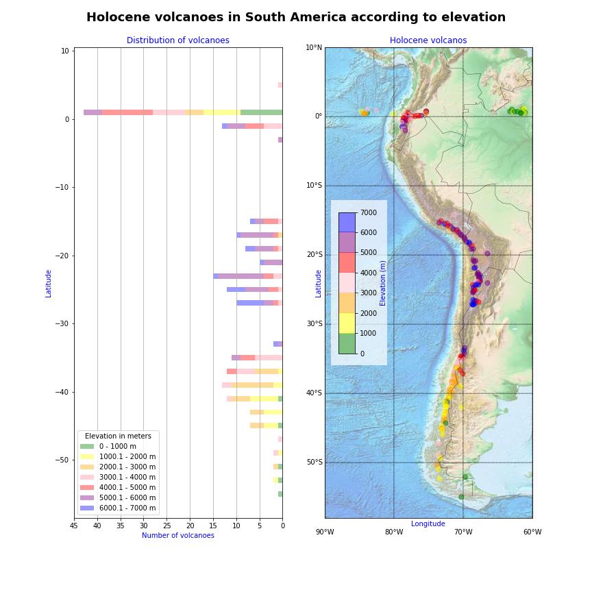
89 A