Tree identification from Terrestrial Laser Scanning data

Transkriptio

1 Juuso Hallikainen Tree identification from Terrestrial Laser Scanning data Diplomityö, joka on jätetty opinnäytteenä tarkastettavaksi diplomi-insinöörin tutkintoa varten. Espoossa Valvoja: Professori Matti Vaaja Ohjaaja: Petri Rönnholm

2 Aalto University, P.O. BOX 11000, AALTO Abstract of master's thesis Author Juuso Hallikainen Title of thesis Tree identification from terrestrial laser scanning data Master programme Geoinformatics Code ENG22 Thesis supervisor Prof. Matti Vaaja Thesis advisor(s) D. Sc. (tech.) Petri Rönnholm Date Number of pages 57+5 Language English Abstract The requirements for more accurate and up-to-date spatial data increases constantly due to changes occurring in the environment. In addition, there is a technical and economical need to map trees, tree ages and sizes, as well in wide forest areas as park areas in cities by modern scanning techniques. The aim of this thesis was to investigate different positioning methods for terrestrial laser scanned trees. The second aim was to examine different techniques to identify the species of the positioned trees. Laser scans from two separate relatively small woodlands were acquired for the thesis. These scans were utilised for tree locating and species identification. Tree positioning was based on the cylinder fitting method performed for tree stems provided by the scans. The results achieved by the positioning were analyzed based on the comparison to the manually measured reference values. To identify the tree species, the tree intensities and structure parameters extracted from the point clouds were used. According to the study results, the classification of some tree species was relatively well succeeded. However, the identification of some other species did not succeed as expected. The best classification correctness of 80 percent was achieved using the combination of tree intensities and the structure parameters, as well as by the structure parameters only. Classification using the intensities only provided considerably more unreliable results. Instead of that, one tree species (spruce) identification succeeded perfectly in each case. However, tree positioning succeeded obviously well, so the tree locations deviated slightly from the reference values. This examination indicated that a reliable evaluation of the tree classification results did not fully succeed with the relatively small tree sample size used in this thesis. To obtain more reliable estimate of success rate for the results provided by terrestrial laser scanning data, a larger sample size may be required. Furthermore, the laser scans for this work were performed in autumn when there were no leaves in the trees. This, of course, affected the intensity-based tree classification. However, modern tree positioning and classification methods appear quite promising. The future use of these techniques require further development and examination work. Keywords Terrestrial laser scanning, Tree positioning, Tree species identification

3 Aalto-yliopisto, PL 11000, AALTO Diplomityön tiivistelmä Tekijä Juuso Hallikainen Työn nimi Puiden paikannus ja lajitunnistaminen maalaserkeilausaineistosta Maisteriohjelma Geoinformatiikka Koodi ENG22 Työn valvoja Prof. Matti Vaaja Työn ohjaaja(t) TkT Petri Rönnholm Päivämäärä Sivumäärä 57+5 Kieli Englanti Tiivistelmä Yhä tarkemman ja ajantasaisen paikkatiedon tarve kasvaa jatkuvasti ympäristössä tapahtuvien nopeiden muutosten myötä. Tämä näkyy myös teknistaloudellisena tarpeena kartoittaa puulajeja, niiden ikää ja kokoa mm. erilaisilla nykyajan keilausmenetelmillä, niin laajoilla metsäalueilla kuin kaupunkien puistoalueilla. Tämän työn tavoitteena oli tutkia maastolaserkeilattujen puiden erilaisia paikannusmenetelmiä. Toisena tavoitteena oli tarkastella paikannettujen puiden lajitunnistusmenetelmiä. Työn toteuttamiseksi suoritettiin laserkeilauksia kahdella erillisellä pienehköllä metsäalueella. Näitä keilausaineistoja käytettiin puiden paikantamiseen ja lajitunnistukseen. Paikannus perustui keilausten tuloksena saaduille puun rungoille tehtyyn sylinterisovitusmenetelmään. Laskennalla saatuja tuloksia analysoitiin vertaamalla niitä referenssiarvoihin, jotka saatiin pistepilvistä manuaalisesti mittaamalla. Lajitunnistuksessa käytettiin puista saatujen pistepilvien intensiteettejä ja rakenneparametreja. Suoritetun tarkastelun perusteella joidenkin puulajien tunnistaminen onnistui melko hyvin. Kaikkien puiden tunnistaminen ei kuitenkaan onnistunut odotetulla tavalla. Käyttäen pistepilvien intensiteettien ja pistepilvistä saatujen puiden rakenneparametrien yhdistelmää, sekä pelkkiä rakenneparametreja, tulkittiin parhaimmillaankin noin 80 prosenttia tuloksista oikein. Pelkkiä intensiteettejä käyttäen saatiin huomattavasti epäluotettavampi tulos. Sen sijaan yhden puulajin (kuusen) tunnistaminen onnistui kaikissa tapauksissa täydellisesti. Toisaalta, suoritetussa tarkastelussa puiden paikantaminen onnistui kokonaisuudessaan hyvin, sillä laskennalla puille saadut sijainnit poikkesivat referenssiarvoista kauttaaltaan varsin vähän. Tarkastelu osoitti, että maalaserkeilattujen puiden tunnistaminen tässä työssä käytetyllä suhteellisen pienellä otoskoolla ei täysin onnistunut. Tarkempi arvio maalaserkeilausaineistosta saatujen tulosten onnistumisprosentista olisi edellyttänyt suurempaa otoskokoa. Lisäksi puiden laserkeilaukset tehtiin syksyllä, jolloin puissa ei ollut lehtiä. Tämä tietenkin vaikutti puiden tunnistamiseen intensiteettien avulla. Nykyiset puiden tunnistusmenetelmät vaikuttavat kuitenkin kokonaisuudessaan varsin lupaavilta. Menetelmien hyödyntäminen edellyttää yhä tutkimus- ja kehitystyötä. Avainsanat Maalaserkeilaus, puiden paikantaminen, puulajitunnistus

4 Preface This Master s Thesis was carried out for Aalto University, Department of Built Environment. The purpose was to study some 3D-techniques utilised in forest mapping to get precise information about forest composition. I like to thank my supervisor Professor Matti Vaaja and advisor Sc.D (tech.) Petri Rönnholm. They have given me valuable guidance, feedback and encouragement. Also, I like to thank Research Assistant Sami-Petteri Karvonen for great support in performing the measurements as well as in preprocessing the data collected by measurements. Many thanks also to my parents, brother and friends working as a good support network during my whole studentship. They have given me valuable encouragement, and guided me in many fundamental issues concerning my studies. Thus, I have got excellent conditions to move towards new challenges. Espoo Juuso Hallikainen

5 Table of contents Abstract Tiivistelmä Preface Table of contents Abbreviations 1 Introduction Terrestrial laser scanning Pulse-based laser scanning Phase-based laser scanning Laser scanning of a forest sample plot Tree location Simple point-based methods Voxel-based methods Extraction-based methods Hybrid methods Tree species identification methods Intensity-based methods Methods based on tree structure parameters Experimental work for tree identification Materials Methods Tree positioning Identification of tree species Results Tree locations and DBHs Tree species classification Analysis Conclusions References Appendix 1. Matlab-code for tree species classification

6 Abbreviations CT DBH DBM DT-CWT DWT ETS FLBH GNSS HLS ICP ID IMU K-NN LCS LLS LS LOOCV MSAC PCA RANSAC RCWF RGB SVM TIN Contourlet transform Diameter at breast height Deep Boltzmann machines Dual-tree complex wavelet transformation Discrete wavelet transform Explicit tree stucture Height of the first live branch Global navigation satellite system Highest branch within crown lower surface Iterative closest point Identification number Inertial measurement unit K- nearest neighbour Longest cross-spread of crown cover Lowest branch within crown lower surface Longest spread of crown cover Leave-one-out-cross-validation M-estimator sample consensus Principal component analysis Random sample consensus Rotated complex wavelet filters Red green blue Support vector machine Triangulated irregular network

7 1 1 Introduction Throughout the years, forests have been highly important for Finland. The reasons for this are obvious: 73 percent of Finnish ground area is covered by forests, making it the most forest-covered country in Europe. Consequently, forests are a source of considerable income for the Finnish economy. In addition, forests are significant for recreational use and climate change mitigation. Thus, forests in Finland are utilised by many organizations from the wood industry to tourism businesses. (Luke 2018; Hetemäki & Hänninen 2013, 204) To increase productivity, the forest industry needs more and more detailed information about the woodland they utilise. For instance, this information includes the location of individual trees and even their species. These data are fundamental part of updated data utilised for forest use planning. For example, a certain forest area can be defined by its productivity and the economical value. (Holopainen et al. 2011a, , 132, ) Furthermore, to find the vendible trees, information about tree heights and age distribution are needed. Usually, the forests need to be thinned out after the trees are metres in average height. The different tree species in turn become harvestable at different ages depending on growing environment and conditions. For instance, silver birches can be thinned already at the age of 20 years, whereas pines often should be several decades older. (Metsälehti 2019) Moreover the crucial parameters used in the evaluation of the woodlands and single trees are diameter at breast height (DBH), defining the basal area and wood volume. (Metsäkeskus 2019, 16-25) Forest inventorying is also needed for the classification of trees according to their growing environment. During the 20th century, nature-based tourism has increased dramatically in Finland. This, in turn, has raised the status of the forests also from the viewpoint of traveling and spending free time. (Holopainen et al. 2011a, ; Hetemäki & Hänninen 2013, ). One example of forests used for recreation is conservation areas. These types of forests comprise natural woodlands (i.e., forests grown without human activities) and are protected by nature conservation law. Protected forests cover 2.7 million hectares, which corresponds to 12 percent of whole Finnish forest area. Based on Finnish law, even 2.4 million hectares of this protected forest area are conserved. (Metsälehti 2019; Luke 2019) In Finland and all over the world, forests are constantly mentioned in headlines about climate change. The importance of forests is underlined due to their importance as carbon sinks and, thus, as climate change mitigators. The growth of the trees significantly absorbs carbon from the atmosphere. To affect the amount of different greenhouse gases in the atmosphere, more information about the composition and the density of forests is needed. Knowledge about the capability of different tree species to absorb carbon and other greenhouse gas components is also essential. (Hiltunen et al. 2018, 5, 6, 8 and 10; Åkerblom et al. 2017, 1) Due to economical and environmental changes, the significance of the rapid and comprehensive forest information collection is increasingly emphasised in forest mapping. During the last decade, laser scanning methods have been developed and have become an

8 2 essential technique in forest mapping. Remote sensing technologies have enabled the mapping of wide forest areas. The spectral data collected by remote sensing methods provide information about woodland composition. However, single trees of the same species may yield slightly different spectrums due to variations in crown shape. Consequently, the identification of individual trees requires more exact methods providing knowledge about the lower part of the tree. This can be performed by terrestrial laser scanning, which enables defining specific geometrical tree parameters. This information can be used as reference data for the accurate estimating of remote sensing material. (Othmani et al. 2013, 1; Lin & Herold 2016, , ) Laser scanning can be performed by aerial, terrestrial, mobile, and personal systems. Aerial laser scanning refers to the surveying of the earth and the different ground targets from above. This can be performed by airplane, helicopter, or spacecraft. By contrast, terrestrial laser scanning refers to the scanning of objects from fixed locations on the ground. Scanning on terrain can also be implemented by mobile systems such as a car or another corresponding vehicle. Recently, scanners have been developed also for personal use. These can be mounted, for instance, on a backpack. The most significant benefit of this scanning method is the independency of terrain conditions. (Cronvall et al. 2012, 13-16) The main advantage achieved by terrestrial laser scanning is a highly dense and explicit point cloud due to the short scanning range and the high angle resolution of the method. (Lin et al. 2010, 1867, ; Kukko 2013, 18; Holopainen et al. 2011b, 5-6; Cronvall et al. 2012, 16) To guarantee reference data with as high accuracy as possible, this study was limited to terrestrial laser scanning. Thus, this work did not focus on the other sorts of laser scanning methods. Tree parameters calculated from terrestrial laser scanning data can be utilised for statistical interpretation. This can provide reliable results that can be combined with specific tree species. Furthermore, the extraction of different tree species from a point cloud produced by laser scanning can be completed by computational algorithms. However, deficiencies continue to exist concerning the methods discussed here. Consequently, the current accuracy and quality requirements could benefit from further development. (Othmani et al. 2013, 1; Lin & Herold 2016, , ; Åkerblom et al. 2017, 4 11) The first aim of this thesis was to examine different approaches to define single tree locations from terrestrial laser scanning data. The second aim was to study different methods to identify the species of the positioned trees. Furthermore, the objective of the thesis was to evaluate the reliability of these methods and the quality of the end results. The goal of the thesis was to answer the following questions: How can a tree be positioned from fixed stations by using terrestrial laser scanning data? How can tree species be identified from the point cloud data produced by terrestrial laser scanning?

9 3 2 Terrestrial laser scanning In contrast to the electromagnetic spectrum that consists of different wavelengths, laser radiation covers high energy waves of the same length. The high efficiency of the laser also enables this method to be used in long-range measurements. The purpose of modelling by laser scanning is to obtain information about the locations of different targets. Spatial data are defined based on the distance measurements between the target and the laser scanner. These distances can be determined by laser signal time-of-flight, which can be achieved by pulse-based or phase-based systems. (Wehr & Lohr 1999, 68-73; Holopainen et al. 2011a, ; Fröhlich & Mettenleiter 2004, 8) In pulse-based scanning, time is registered directly by the receiver of the scanner. In phase-based scanning, the phase difference between the outgoing and returning signal is transferred to the time difference. The main components of the laser scanner are the laser transmitter, ranging unit, i.e., the laser reflecting mirror and the receiver. (Wehr & Lohr 1999, 68-73; Holopainen et al. 2011a, ; Fröhlich & Mettenleiter 2004, 8) Laser scanning can be accomplished by single- or multi-scan operation from the same area. (Liang et al. 2011, 38) Figure 1: Terrestrial laser scanner. (Wang et al. 2019a, 6) Terrestrial laser scanning refers to scanning acquired on the ground from fixed stations. The main components of the system are the scanning instrument, tribrach, tripod, and power supply (an accumulator or network power) (Figure 1). Terrestrial laser scanners can be equipped with or without internal memory. In case the internal memory does not

10 4 exist, a separate computer with memory is needed. The scanning is performed either from a single or several stations depending on the target of the mapping. The advantage of the single-station operation is the low amount of point cloud data and, thus, the rapid processing of the information. (Cronvall et al. 2012, 16; Holopainen et al. 2011a, ; Oveland et al. 2017, 1-3) However, the disadvantage of this method is that scanning from one point does not cover gap areas behind the trees. In addition, this method does not allow a dense point cloud to be established from targets lying dozens of metres away. Thus, the modelling of all individual tree trunks may not be feasible. Consequently, specifying single tree locations and the DBH is challenging and may even be impossible. Therefore, the mapping of a forest area usually requires scanning from several stations. The scanning results are typically registered into a common point cloud. (Cronvall et al. 2012, 16; Holopainen et al. 2011a, ; Oveland et al. 2017, 1-3) The advantage of terrestrial laser scanning is the high density of the point cloud achieved by the technique. The cloud density may be as many as tens of thousands of points per square meter. The disadvantage of the method is cost inefficiency due to immobility. On the other hand, the density of the point cloud accomplished by terrestrial laser scanning depends on scanning distance. This range can vary from metres to hundreds of metres. Furthermore, the angle resolution, the capability of the scanner to detect details, is a key factor when evaluating the scanning applicability. A more accurate angle resolution guarantees a higher point cloud density, and thus, also smaller objects are detectable from the point cloud. (Lin et al. 2010, 1867, ; Kukko 2013, 18; Holopainen et al. 2011b, 5-6; Cronvall et al. 2012, 16) 2.1 Pulse-based laser scanning Pulse-based laser scanning is based on the laser time-of-flight. This time consists of laser delay from the laser scanner to the target and back to the scanner. The time-of-flight is registered by the receiver (Figure 2). Thus, the distance R between the scanner and object can be calculated according to Equation 1. (Wehr & Lohr 1999, 69-73) R = 1/2 c t L (1) In this equation, symbol c is the speed of light and tl is the time-of-flight of the laser signal. Every laser scanning instrument has a time resolution tl, which is the minimum time space registerable by the receiver of the scanner. Consequently, the range resolution R of the laser instrument is definable according to the Equation 2. (Wehr & Lohr 1999, 69-73) R = 1/2 c t L (2) Pulse-based laser scanners are usually applied in scanning operations extended with a range from a few metres to two kilometres. The largest bottleneck of pulse-based scan-

11 5 ning operations is the time gap between the laser beams reflected to the scanner. Consequently, the pulse-based scanning may be unprofitable in short-range measurements. (Holopainen et al. 2011a, ; Fröhlich & Mettenleiter 2004, 3, 8; Cronvall et al. 2012, 12; Alho et al. 2011, 3) However, the advantage of the pulse-based method compared to the alternative phasebased ranging is the lower sensitiveness to noise. Thus, pulse-based scanning can also be applied in short distance measurements. (Liang et al. 2018, 155; Bartolo & Salvini 2019, 5) Furthermore, the scanners have a maximum range. This distance can be calculated using Equation 3 applying the maximum time the scanner is able to register. (Wehr & Lohr 1999, 69-73; Cronvall et al. 2012, 12) R max = 1 2 c t max (3) The range depends on the effect of the send laser pulse and the highest time-of-flight defined by the repeating frequency of the measurement. (Wehr & Lohr 1999, 69-73; Cronvall et al. 2012, 12) However, Equation 3 is theoretical. In practice, the performance of the laser beam is sensitive to the circumstances. The foremost distractions affecting to the laser signal are signal noise and the reflection from the different targets. Consequently, the accuracy of the laser scanning can be defined by Equation 4. 1 σ R ~ c t 2 rise (4) ( S N ) In this equation, trise is the rising time of the signal, S is the signal power without the noise, and N is the power of thermal noise. (Wehr & Lohr 1999, 69-73) Figure 2: The principle of pulse-based laser scanning. (Wehr & Lohr 1999, 70)

12 6 2.2 Phase-based laser scanning Phase-based laser scanning comprises the solving of the phase difference between the outgoing and returning modulated signal (Figure 4). The laser beam is modulated by at least two different wavelengths onto one signal (Figure 3). In this signal, the longer modulation wave consists of shorter modulation waves. Thus, the longer wavelength can be defined as the function of shorter wavelengths. Consequently, millimetre-level accuracy can be achieved by phase-based scanning in longer range measurements. The signal traveling time tl can be solved by applying Equation 5. Here, φ is the phase difference between the leaving and returning laser signal, T is the period length of the signal wave, and n is the integer amount of the periods in question. (Wehr & Lohr 1999, 69-73; Alho et al. 2011, 3; Pfeifer & Briese 2007, 6-7) t L = φ T + n T (5) 2 π Figure 3: The principle of amplitude modulation. (Pfeifer & Briese 2007, 6) As the frequency f is the inverse of the cycle duration, Equation 5 can be also written as Equation 6. This equation, in turn, can be substituted into Equation 1 when the phase difference is transformed to the signal time-of-flight. Thus, the range between scanner and target can be defined by Equation 7. (Wehr & Lohr 1999, 69-73; Alho et al. 2011, 3) t L = φ 2 π 1 f (6) R = 1 4 π c f φ (7) By utilising the different wavelengths covered by the laser beam, the shortest and the longest measurable distance of the scanner can be defined. In Equation 8, φ is the minimum and in Equation 9, λ is correspondingly the maximum available signal wavelength. (Wehr & Lohr 1999, 69-73; Alho et al. 2011, 3) R = 1 4 π c f φ (8)

13 7 R max = 1 4 π c f 2 π = λ 2 (9) Figure 4: Outgoing and returning laser beams, as well as their phase difference. (Wehr & Lohr 1999, 71) Phase-based laser scanners are applied in terrestrial and other short-range measurements that usually are under 100 metres. Due to its signal consistency, the technique is quite cost-effective. Thus, a signal without time gaps guarantees a dense point cloud. For example, at the distance of 10 metres from the laser scanning instrument, even 25,000 points can exist per square meter. (Fröhlich & Mettenleiter 2004, 8; Holopainen et al. 2011a, ; Alho et al. 2011, 3) 2.3 Laser scanning of a forest sample plot Single-scan terrestrial laser scanning refers to the mapping of a forest sample plot from one station (Figure 5(a)). A sample plot covering 3D-model can be achieved by this operation. This method enables to define the locations and the DBHs of the trees covered by the plot. Typically, the scanner rotates 360 degrees in the horizontal direction, while the field of view in the vertical direction is 300 degrees. (Liang et al. 2011, 38, 46) The advantage of single scanning is the low amount of data. Consequently, also the time needed for data processing is relatively short. (Liang et al. 2016, 66) The sample area is well measurable within 20 minutes. This time conventionally covers the setting of the scanner and the performing of the scanning. The setting usually takes 2 10 minutes, while the scanning takes 5 10 minutes. However, the disadvantage of the operation is its incompleteness. Easily over 40 percent of the tree stems covered by the

14 8 sample plot are occluded. Thus, the results achieved by the 3D-point cloud are not explicit. The percentage of the gap areas increases as the ranging distance increases. This issue is especially emphasised in dense forests. (Liang et al. 2016, 66) However, this type of laser scanning may be cost-efficient depending on the mapping environment. For instance, for forest plots only comprising single tree species, the single scanning can be quite profitable. Over 80 percent of trees located within the radius of tens of metres from the scanner can be detectable. Tree extraction and location are performable based on automatic algorithms. (Liang et al. 2011, 38-39, 45) Figure 5: (a) Scanning performed from a single location (single-scanning). (b) Scanning performed from several locations, wherein the laser point cloud is registered using the artificial targets (multi-scanning). (c) Scanning performed from several locations, wherein the laser point cloud is registered at the feature level using the tree stems (multisingle-scanning). The black circles indicate the mapping area. The red rectangles locating on the circles and in the middle of them correspond to the scanning stations. The purple ellipses inside the circle symbolise trees to be mapped, and in Figure (b) the blue stars indicate artificial targets. (Retelled Liang et al. 2016, 66) Scanning performed by a single scanner can also be complemented by using several scanning stations (Figure 5(c)). This surveying method is called multi-single-scanning. The procedure also enables modelling and positioning of the occluded trees. The scans are registered to a common coordinate system at the feature level displaying the single trees. To locate the trees from the sample plot, XYZ-coordinate system is defined for the point cloud. In this system, the position of the centre scanning station is selected as the origin. (Liang et al. 2016, 66-67) The advantage achieved by the method is the relatively short time required by the collection and the registration of comprehensive point cloud data. Furthermore, the effect of the weather conditions on the multi-single scan method is quite low. In windy weather, the swaying trees follow each other, and thus, the swaying does not influence on the explicitness of the registered data. However, the multi-single scanning process may not be accurate enough to define non-spatial properties, such as species. Gaining information about these properties typically demands scanning procedures using artificial targets. (Liang et al. 2016, 66-67, 71; Dassot et al. 2012, 87)

15 9 This scanning is called a multi-scanning operation. Conventionally, surveying comes into question when a highly explicit and detailed point cloud is desired. The significance of the method is especially emphasised when knowledge about the tree species composition of a dense forest is needed. Surveying is performed from several scanning locations as in the multi-single-scanning operation. The most considerable difference compared to the previous method is the artificial targets applied for the registration of the point cloud (Figure 5 (b)). These reference targets are usually spherical objects placed to the plot at suitable distances referred to each other. (Liang et al. 2016, 66; Dassot et al. 2012, 87) The centre of the reference targets are approximated from the first point cloud (i.e., the scan at the plot centre). Next, the other scans are registered to the same coordinate system using the targets. The purpose of multi-scanning method is to accurately survey and model each tree in the sample plot to define the tree species. However, the multi-scanning operation takes considerably longer than previous methods. Compared with the multisingle-scanning operation, another practical difference is the number of required equipment. The previous method only requires one scanner and a tripod. (Liang et al. 2016, 66; Dassot et al. 2012, 87; Liang & Hyyppä 2013, 1627; Wang et al. 2019b, 135) Instead of that, multi-scanning surveying demands several tripods and reference spheres in addition to the single scanner. One registration sphere is mounted to each tripod, and the scanner is moved between the tripods to take each scan. The essential number of tripods and spheres depends on the area and the tree composition of the sample plot. (Liang et al. 2016, 66; Dassot et al. 2012, 87; Liang & Hyyppä 2013, 1627; Wang et al. 2019b, 135) The disadvantage of the multi-scanning survey is the high costs derived from time consumed for equipment set up and registration, as well as the processing of the data. The registration and other manual operations may take significant time. A scanning operation consisting of the setting up the scanner and targets, as well as scanning from five stations, can easily require one hour. Moreover, completing the whole process demands a minimum of two persons, whereas the multi-singe-scanning and single-scanning operations mentioned above require only one person. (Liang et al. 2016, 66-67; Liang & Hyyppä 2013, 1627) Staff members are needed to speed up the procedure, such as carrying all tripods, reference targets, and scanners to the plot, as well as to setting up the scanning network. (Liang et al. 2016, 66-67; Liang & Hyyppä 2013, 1627) Furthermore, the weather conditions may set significant constrains for the multi-scanning method. For instance, wind causing wide sways to the tree crowns may disrupt the registration of the scans. (Liang et al. 2016, 66-67) 3 Tree location 3.1 Simple point-based methods Oveland et al. (2017) reported in their article a mobile laser scanning process. In this technique, the tree positioning is based on the definition of the stem DBH and stem centre

16 10 location. The process is accomplished as illustrated in Figure 6. In this operation, the position and tilt of the angles of the laser scanner in X-, Y- and Z-coordinates are first determined using global navigation satellite system inertial measurement unit (GNSS- IMU). (Oveland et al. 2017, 5 9; Koska et al. 2018, 136) Figure 6: The definition of tree locations. (Oveland et al. 2017, 5) The heights of the points in the laser point cloud are derived from these data. These point heights are transformed from the local scanner coordinate system to the universal one. The next step is cloud classification. The cloud can be classified to tree stems, ground, or not classified points. The classification to the same object is based on the threshold describing the increase of the distance measured by the laser scanner. If the distance difference between neighbour points does not exceed the threshold, the points belong to the same object. Furthermore, point classification for tree stems requires that the maximum value is set to the DBH of the stem. (Oveland et al. 2017, 5 7) If the distance increases by subsequent rangings not exceeding the threshold and the horizontal distance exceeds the maximum allowed DBH, the points are classified as the ground. The points will stay unclassified if the distance between two subsequent measurements is exactly equal to the threshold. (Oveland et al. 2017, 5 7) After the classification, the DBH and the coordinates of stem centre are defined by applying the circle-fitting algorithm using the least squares method. The method fits a circle by undergoing coordinates of every point classified as tree stems and thus searching for a constant centre and radius of the stem. (Oveland et al. 2017, 5 7; Bucher 2004) The multi-layer scanner rotates not only in horizontal direction but also, to some extent, in vertical direction depending on the number of laser channels. There is always some known vertical angle between the subsequent channels. Consequently, there must be enough circles and their centres found by the fitting method also in vertical direction to classify them as tree stems. (Oveland et al. 2017, 5 7)

17 11 The next step is to enhance the registration of the point clouds measured from different locations by applying iterative closest point ICP-algorithm. Moreover, this method allows to improve the accuracy of the stem centre coordinates defined by circle fitting. The ICPalgorithm forms pairs from the consecutive point clouds. The second cloud of the pair is registered to the first cloud by fitting the points to each other by shifts and rotations. The current and original cloud form a new reference point cloud. The same registration process is continued until all data is registered to the same coordinate system. (Oveland et al. 2017, 5 7) As the GNSS-signal under the canopy cover is easily defective, the correction of data is required to define tree stem location in the common coordinate system. After the circle fitting, the correction of terrain and tree height data is accomplished. The correction is performed by registering the mobile laser scanning data to the airborne laser data collected from same area. First, the height differences between the ground points of these data sets are considered. According to the comparison, the ground mobile laser scanning points are more accurate than upper mobile laser scanning points. Thus, the more reliable points are registered to the airborne laser scanning points comprising the GNSS-data. Consequently, the DBHs and the tree locations in the ground coordinate system are definable. (Oveland et al. 2017, 5 9) The DBH is defined based on a model representing the stem diameter estimated from the mobile laser data as the function of stem height. According to this model, the stem diameter can decrease, for example, one centimetre per meter from the root of tree. In the end, the average stem width and the centre position is derived by clustering the points within a particular maximum distance. (Oveland et al. 2017, 5 9) Koren et al. (2017) presented in their article other mathematical operators applicable to define the location and DBH of trees. The tree coordinates can be derived based on, for instance, the minimum bounding box method. With this method, the cross-section of the tree is bounded by a cuboid at breast height. The bounding is completed by the box covering only the minimums and the maximums of stem X- and Y-coordinates. Based on the average of these coordinates, the stem location can be determined. (Koren et al. 2017, 124; Chernov & Lesort 2005, ) Moreover, the tree position is definable from the average of X- and Y-coordinates of points corresponding to the stem cross section. Furthermore, the stem coordinates are derivable from the average of the outermost point locations. The next step is to calculate the DBH using the distances from the defined stem centre point to each cluster point. Thus, the DBH is achievable as the result of doubling the average of these distances. (Koren et al. 2017, 124; Chernov & Lesort 2005, ) Using the methods mentioned above, the tree locations and DBH can be initialised. These values are improvable by the previously mentioned least square method and the Monte Carlo -method. This process is based on the random values achieved by the initial methods. A minimum number of points corresponding to the trunk cross-section is randomly chosen for the initial circle fitting. The centre coordinates and the radius of the fitted circle are determined. The squared errors between each trunk point and the fitted circle are sorted in the ascending order. Thereafter, n number of the points corresponding to n lowest ordered residuals are selected for the circle approximation. The same initial procedure is repeated until a particular maximum limit is reached or the desired accuracy is

18 12 achieved. (Nurunnabi et al. 2018, ; Koren et al. 2017, 124; Chernov & Lesort 2005, ) 3.2 Voxel-based methods Tree location can also be defined based on voxelization methods. The procedures consist of terrain model estimation and tree height normalization, as well as tree stem voxelization. Depending on the form of the ground, the terrain model can be estimated based on either the heights of the closest neighbours in the laser point cloud or the heights of each separate point. In the first estimation method, the terrain is divided into square cells in a horizontal direction. (Cabo et al. 2018, ) Thereafter, the lowest point inside each cell and its eight nearest neighbours are examined. If the height difference between the lowest and neighbour points exceeds the threshold describing the variety of the terrain model, this cell is updated as the lowest of the ground. In the alternative height-normalization method, the point cloud representing the forest plot is projected to a flat surface based on the height difference between the ground and non-ground points. After the height-normalization, the point cloud is vertically bounded into a slice covering the tree stems so that they are detectable (Figure 7). The stems must not be occluded by the branches or the undergrowth. (Cabo et al. 2018, ) Figure 7: The tree stems are separated in the interval in which they are not occluded. (Cabo et al. 2018, 167) The bounded point cloud is divided into voxels (i.e., small cuboids). There is always some points in the centre of the cuboid. The same cuboid can consist of several points. Consequently, a randomly distributed point cloud can be modified as a homogenous and simple data set comprising as little redundant data as possible. Thereafter, the coordinates of the laser points are defined in the voxel system. These coordinates enable the determination of the DBHs and the coordinates of the stem centres. (Cabo et al. 2018, ; Cabo et al. 2014, 48-50) Furthermore, the voxelization can be performed by using the octree algorithm. This algorithm divides the original point cloud into cells. One point is randomly selected from each cell. The ground points are picked up by the morphological filtering method. This algorithm uses a 1-dimensional line or 2-dimensional mask approximating the minimum

19 13 (Zmin) and maximum height (Zmax) in the XY-level. The operation is based on the dilation of the filtering mask. The mask is dilated until the height difference between the points inside the mask are high enough. Then, the lower points within the mask are classified to the ground. Thus, the observation of the trees from the terrain is possible. (Liang et al. 2018, 173; Zhang et al. 2003, 873) The tree detection is based on the combination of the tree voxels in the horizontal and vertical directions. Each point is gone through and clustered in the voxel system by the octree-algorithm. The clustered voxel space enables to find the links from the tree in the vertical direction. More than one link from the neighbour voxels are searched. The searching of the connections can be performed by traversing each voxel at each tree level from the ground level to the top or vice versa. Thereafter, the noise is filtered from the clusters. The filtering is based on the assumption that all point neighbourhoods follow the Gaussian distribution with a known threshold. Finally, the DBH of the tree is defined by cylinder fitting in particular vertical intervals. The centre of the cylinder approximated by these vertical slices corresponds to the tree location. (Liang et al. 2018, 173) 3.3 Extraction-based methods Tree positioning can also be performed by stem fitting. The first step before performing this method is tree extraction by eigenvalue decomposition. This technique is based on the point cloud coordinate transformation between the terrain and tree stem. The decomposition determines the eigenvalues of the new (i.e., stem coordinate system). The aim of the decomposition is that the deviations from the X- and Y-axes in the transformed point cloud are minimised. The eigenvalues enable the calculation of flatness values to different objects. A low flatness value refers to lower objects, typically the terrain, and high value correspondingly to higher objects such as the trees. (Liang et al. 2012, ) After tree extraction, the tree stems can be modelled. Stem modelling is completed by cylinder fitting to the stem points. The cylinder is fitted based on the normal of the stem surface achieved by the eigenvalue decomposition. The possible curve of the stem is considered in the fitting based on the stem radius and its direction. The final cylinder fitting is performed by minimizing the square sum of the residuals between the fitted cylinder surface and laser points. The standard deviation calculated by the minimal residuals enables Tukey s estimator to be defined. This parameter reduces the weight of the error caused by larger outlier points from the cylinder. Consequently, the deviation of the tree from the vertical direction is better known. Thus, tree location can be also more accurately determined. (Liang et al. 2012, ) In addition, tree extraction can be performed by Hough-transformation. This algorithm is based on circle detection by parameter transformation. The first step in the process is the generation of the elevation model using the ground points registered by terrestrial laser scanning. Two different raster sizes are used for the model generation. The larger rasters aim to cover the terrain, whereas the smaller rasters capture only the trees. After the rasterization, the heights of the points within the smaller rasters are interpolated using the heights of the points inside the larger rasters. (Olofsson et al. 2014, ; Gonzalez & Woods 1992, )

20 14 The points are classified into the terrain or the trees according to the height threshold. If the interpolated value of the point exceeds the threshold, the point is classified as the tree. Correspondingly, if the value is under the threshold, the point is classified as the terrain. Tree location is performed in the raster field from one to two metres in the vertical direction. The ratio between the registered laser pulses and overall laser pulses inside the raster neighbourhood is determined. Value zero for the ratio refers to the nonexistent reflections from the breast height in the neighbourhood. Correspondingly, value one refers to the reflections of all laser pulses from breast height. Based on these values, the existing probability of a tree in each raster neighbourhood is definable. The tree location is the raster with the highest existing probability in the neighbourhood. (Olofsson et al. 2014, ) The point cloud representing the positioned tree is classified into the stem and the terrain. Classification to the stem is based on the bounding of the point set with a box consisting of the stem and a part of the crown. Thereafter the bounded point data is divided into the rasters with normalised intensity values from 0 to 255 according to the number of points. To reduce the noise, some threshold value is chosen from this space, and the values below the threshold are classified to zero. (Olofsson et al. 2014, 4329) The next step is the extraction of the tree stem radius based on the Hough-transformation. This algorithm examines each pixel belonging to the trunk and fits the initial circles to these pixels. The equations of the initial circles are transformed into the parameter space of the circle central angle, revealing potential circles. Next, the circle representing the stem is chosen according to the number of intersections between the found circle candicates. The circle with most intersections with the other circles corresponds to the tree trunk (Figure 8). The process is started from the trunk height of one meter, and the radiuses are extracted until approaching the crown, which changes the results significantly. (Gonzalez & Woods 1992, ; Olofsson et al. 2014, ) Figure 8: Coloured circles corresponding to the tree stem according to the Hough-transformation. The red circle intersecting with most of the other circles corresponds to the tree stem most closely. (Olofsson et al. 2014, 4330)

21 15 Classification into the crown with a random sample consensus (RANSAC) based method is performed by searching for the first pixel deviating from the value of the stem. The pixel is searched by following the stem in the vertical direction. Next, the points of the trees corresponding to the extracted radiuses are considered. This procedure is based on the default that the distance between the centres of the extracted trees and other points corresponds to the same trunk if the distance is below the product of 1.5 and the determined radius. The final result for the DBH is defined by the RANSAC-algorithm. This technique describes the number of repetitions providing a certain model representing the diameter of the tree stem by a particular probability. The DBH is approximated by an appropriate RANSAC-value, and finally, the stem location is determined in the common coordinated system by fixing it to the GNSS. (Olofsson et al. 2014, ) In addition, calculational processes to detect stems can be used. The simplest cases, such as a point cloud representing a forest plot achieved by the single-scanning method, enable the extraction of the stems by computational methods in 2D space before filtering of the stems. Correspondingly, the extraction of the trees from a point cloud achieved by multisingle scanning may be computationally more time- consuming. The models like this can be difficult to modify as enough whole data sets. Moreover, noise filtering or eliminating redundant data may destroy the point of cloud texture. However, the 2D-computation for the point data set achieved by a single-scanning method with the ranging distance of a few dozens of metres may be more effective compared to the 3D-computation. (Liang et al. 2011, 38, 41-45) The extraction of the trees is based on the continuity of the stems. Thus, the points close to each other in 2D- and 3D-point clouds are homogenously distributed especially in objects near the scanner. The distance between the subsequent points further from the scanner is longer than the nearer points due to the decreasing resolution as the ranging distance increases. In addition, the 3D-form of objects influences the point distribution. Consequently, the deviations of points close to each other can be considerable. Furthermore, the branches of the tree crown are easily occluded by each other, causing discontinuity to the 2D-level. However, these factors can be eliminated by computational methods. (Liang et al. 2011, 41-42) The computational tree extraction method described above, can be based, for example, on the point cloud segmentation in horizontal and vertical directions in 2D-data. Each point is traversed in both directions, and the location and distance data of the points are combined. The point classification into the tree trunk is based on the combined point data. The points belong to the trunk if there is enough continuity in the point locations and in the ranging distance between the points (Figure 9). The segmented points are classified to the stem if the distance between the points is below the known threshold values in pixels and centimetres. Furthermore, the pixel size of the classifiable point data must usually have a particular lower limit. The points are not identified as stem points if the pixel size is under the threshold. (Liang et al. 2011, 42).

22 16 Figure 9: (A) The measured height as the function of ranging distance. (B) The measured height as the function of ranging distance corresponding to horizontal distance. (Liang et al. 2011, 42) Furthermore, the scannings performed in upward slope directions skew the results in horizontal directions. These scans cause considerable variance to the vertical tree trunks. Consequently, the tree stem extraction from the points achieved by the upward slope scanning direction requires correction based on the cosine of the scanning angle. (Liang et al. 2011, 42-43) Thereafter, the filtering of the trees from the point cloud is possible. The filtering is based on the separating of subsequent points in the vertical direction because the points further from each other refer to the tree branches and the other parts of the crown. The points are classified into the trunk according to a particular vertical variance. (Liang et al. 2011, 42-43) The point classification to the tree trunk may take place with following conditions. First, each laser points with vertical standard deviation at least double compared to the average distance between the points, are excluded. Second step is to determine the distance between each point in the vertical direction. These points are classified into the trunk according to a particular threshold. If the distance between the points in the vertical direction exceeds the threshold, the stem is regarded as tilted. Thereafter, the trunk is fitted to the point cloud, and the points lying further from the trunk are excluded according to the known limitations (Figure 10). (Liang et al. 2011, 42-43)

23 17 Figure 10: The tree trunk filtering. (A) The tilt of the tree trunk fitted to the point cloud. (B) Appropriate tree trunk for the point cloud according to the distance of the points. (Liang et al. 2011, 43) After the tree stem is classified, stem is modelled based on two steps. First, the trunk fitted to the point cloud is divided into slices with a thickness of 20 centimetres each. The point sets corresponding to these slices are projected to the XY-level (i.e., horizontal direction). The circles are fitted to these point sets based on the least square fitting method. In other words, the perpendicular distances between the point sets and the circle fitted to them must be minimised. If some of the fitted circles and their centres do not match with the vertical/upward slope line corresponding to the centre of the fitted stem, the circles are excluded (Figure 11(E)). Thereafter, the stem position can be determined from the centre of the circle at the DBH. (Liang et al. 2011, 43)

24 18 Figure 11: Laser point cloud processing from the tree extraction to the stem positioning. (A) Tree extraction in the 3D-space based on the point distribution. (B) The trunk extracted from the point cloud. (C) Filtered trunk. (D) Fitted circles to the filtered trunk. (E) The fitted circles deviating considerably from each other are excluded. (Liang et al. 2011, 44) 3.4 Hybrid methods Tree stem positioning can be determined by several previously mentioned methods simultaneously. This techniques are called hydrid methods in general. One example of a hybrid method is the point-based triangulated irregular network (TIN) iteration. The triangles are created from the lowest points of the cloud cell neighbourhood. (Liang et al. 2018, 144) Thereafter, the height between the remaining points and the triangle above them are classified into the tree or the terrain. Half of the point cloud scale is used as the threshold. If the height of the point from the triangle is below the threshold, the point is classified to the ground. The next step is the tree reconstruction based on point cloud voxelization. The points representing the tree trunk are separated from the voxels. Then, the stem curve is estimated based on the circle-fitting algorithm and the Hough-transformation. The stem diameter is defined based on these methods at different heights of the stem and at the DBH, whereby the centre of the fitted circle corresponds to the tree position. (Liang et al. 2018, 144)

25 19 4 Tree species identification methods 4.1 Intensity-based methods Intensity-based methods require some preprocessing. Tree species identification from the laser point cloud can be based on, for example, the 3D-models representing the tree stems. These models can be smoothed by Laplacian transformation. This algorithm calculates the location of each laser point based on the weighted average. The process is iterative, meaning it is repeated as long as the point cloud model requires smoothing. (Othmani et al. 2013, ) The next step in the method is to create a deviation map of the smoothed and original point clouds. The map is created based on the difference of each point between the original and smoothed models. The deviation model is, in turn, projected as a 2D map with the intensity value of each pixel scaled from 0 to 255. (Othmani et al. 2013, ) Thereafter, the deviation map is classified based on the wavelet transformation and curve extractions. The wavelet transformations are based on the filtering of laser point intensities. One of the wavelet transformations is the discrete wavelet transformation (DWT). This method is based on approximation by high- and low-pass filtering. Then, a wavelet function with vertical, horizontal, and diagonal coefficients using the time frequencies, is created. A more improved version of this method is the dual-tree complex wavelet transformation (DT-CWT). This process enables the separation of tree species by the real and the imaginary parts, contrary to the previous procedure based on the real parts only. (Othmani et al. 2013, ) The previous wavelet transformation can also be performed in a 2D-layer (2D DT-CWT). This procedure filters the waves in six different directions. A further improved transformation is 2D-rotated complex wavelet filters (2D-RCWF). Compared with the previous method, this method has twice the number of filtering angles. The combination of these two procedures can be utilised to maximise classification accuracy. The contourlet transformation (CT)-algorithm based on the Laplacian-operator is used for the smooth curve extractions from the natural images. The Laplacian-operator comprises a pyramid dividing the original image to the filtered sub-images (Figure 12). (Othmani et al. 2013, )

26 20 Figure 12: A figure representing the tree species identification based on intensity distribution. (Othmani et al. 2013, 2149) The sub-images provide information about the reflection angles of the intensities. Tree classification based on the geometric features is performed according to the amount of energy coming through each channel. Furthermore, the weighted average and the standard deviation of the outcoming amount of energy is determined to classify the trees. The final classification results are achieved by the decision tree utilising the feature vectors. Twothirds of these vectors identify tree species and the last third defines the classification errors. (Othmani et al. 2013, ) Tree classification into the different species can also be based on the laser intensity waveform. This waveform represents the vertical geometric form of the tree (Figure 13). The tree is vertically divided into a certain number of profiles. Tree classification is performed by a deep learning model, deep Boltzmann machines (DBM). The model is utilised to explore the proportion of the visible and hidden points to the entire number of points in each profile. (Guan et al. 2015, ) Figure 13: Three examples of waveforms provided by mobile laser scanning representing three different tree species. (Retelled Guan et al. 2015, 867) The laser beams are scattered from the trees and other objects, distorting the intensity values registered by the receiver of the laser scanner. In addition, the geometric features of the scanned targets and the scanning distance affect the behaviour of the radiation. Consequently, the intensity must be calibrated. This calibration can be completed, for example, by considering the reflections from a white sphere and comparing them to the reflections from the other objects. In this method, the effect of the laser beam reflected in the angle from 0 to 90 degrees is considered in proportion to the effect of the outgoing laser beam. (Bretagne et al. 2018, 15-19)

27 21 In practice, this calibration is based on four assumptions. First, the laser points appearing on the surface of the calibration sphere are assumed to be very small and do not expand to a wide area. Thus, the intensity of the laser beams is not expected to be decreased when they hit the sphere. Second, the aperture of the laser scanner receiver is assumed to be circular. Thus, the energy registered by the receiver can be defined accurately. Third, each point appearing on the surface of the registration sphere corresponds to the laser beam hit onto the sphere. Fourth, the white sphere is assumed to reflect the entire incoming radiance. This enables the comparison of the radiances reflected from the tree stems to those reflected from the white sphere. When these assumptions are true, the correction for the intensities of the trunks can be performed. (Bretagne et al. 2018, 15-19) Moreover, the visible colour corresponding to the laser wavelength can be utilised in the calibration. The intensity values of the laser points between 0 and 1 can be scaled to the values from 0 to 255. For example, the green-level values can provide information about the chlorophyll of different trees. The chlorophyll data can, in turn, be used in tree species recognition. The effect of the sunlight on the colour values of the laser points is eliminated based on the Illuminant D65 -standard. This standard defines the correlations between the sun illumination and the laser points in proportion to the average daylight illumination. The scaling of the colour values from 0 to 1 into the range of 0 to 255, in turn, is based on the correlation between the illumination and wavelength at a particular bandwidth. (Bretagne et al. 2018, 15-19) 4.2 Methods based on tree structure parameters In addition to the intensity methods, tree species identification can be based on the explicit tree structure (ETS) parameters (Figure 14). The parameters utilised in these methods are tree height, DBH, branch angle, height of the highest branch within the crown lower surface (HLS), and height of the lowest branch within the crown lower surface (LLS). Furthermore, the measurements of parameters with disruptions appearing in the classification method are considered. These errors can consist of, for example, variations in tree stems and ages corresponding to the same species. The aim is to eliminate these errors by, for instance, using optimal parameter combinations to maximise the classification accuracy. (Lin & Herold 2016, )

28 22 Figure 14: (a) Vertical structural dimensions and (b) the maximum and the minimum radius of the tree crown utilised for tree species identification. (Lin & Herold 2016, 109) The combination of the parameters can consist of the radius length corresponding to the tree crown horizontal area (Figure 14(b)) and the variables defined by the earlier mentioned parameters. These quantities describe the tree structure comprising the stem, branches, crown, and leaves (Figure 15). The minor and major axes corresponding to the ellipsoid that approximates the tree crown (Figure 14(b)) is determined by a principal component analysis (PCA). This method bounds the tree crown to an area in which the deviation of the neighbour point data is minimal. The bounded point set is projected to the terrain. (Lin & Herold 2016, 109; Monnier et al. 2012, 246) Figure 15: Definitions and abbreviations for tree structure parameters. (Lin & Herold 2016, 109) The radius of the circle with the same area as the ellipsoid can be defined. Thus, tree structure parameters such as crown length and height, branch angle, and heights of the lowest and the highest branch in the lower crown surface (Figure 14(a)) are definable.

29 23 These quantities can be determined by a segmentation method. This method bounds the point cloud representing the tree structure to the stems, branches, and crown (Figure 16). (Lin & Herold 2016, 109) Figure 16: The tree bounded to different structures by the cylinders. (Lin & Herold 2016, 110) The tree species classification based on the structure parameters utilises the support vector machine (SVM). This procedure separates two tree species based on the tree parameter with the largest difference between the trees. Finally, the classification accuracy is evaluated by the leave-one-out-cross-validation (LOOCV) method. This procedure is combined with the SVM. The LOOCV-SVM -algorithm defines the relation of the correctly classified tree species to the total number of the sampled trees and the number of all corresponding species. These error parameters are considered in the evaluation of classification accuracy. (Lin & Herold 2016, 110) Moreover, the tree identification algorithms based on the structure parameters are k- nearest neighbour (K-NN) and the multinomial regression methods. The former is based on the feature vectors consisting of the structure parameters that correspond to each tree species. The trees are classified into certain species based on the structure parameters corresponding to each known tree. K nearest neighbours corresponding to each parameter are searched, and the feature vectors are constructed from these neighbours. Each classifiable parameter is considered to belong to the majority class of the feature vector element. Thus, the structure parameters of each known tree can be used as reference data for tree classification. (Åkerblom et al. 2017, 4; Yu et al. 2001, 1-5) The existing probability that a feature appears in a certain tree species can also be defined by multinomial logistic regression and logistic regression values. Matlab function Mnrfit creates a regression model between each value of the structural parameter, and their existing probabilities corresponding to the same species. This regression works as a reference model for the regression created by Matlab function Mnrval and identifies the tree species from a wider area. (Åkerblom et al. 2017, 4; Mathworks 2019a; Mathworks 2019b)

30 24 5 Experimental work for tree identification 5.1 Materials The tests for the experimental work of this study were performed in the Otaniemi district of Espoo, Finland during autumn During this time, no leaves were in the trees. This issue affected the results of the experimental work. Figure 17 shows the Otaniemi district with the test area bordered with red line. Figure 17: Otaniemi district with the test area shown with red line. Inside the test area shown in Figure 17, five separate scan registrations were performed. Figure 18 shows these five different plot areas. Three sample plots were scanned without red green blue (RGB) values, plots 1 3, and two plots were scanned with RGB-values, plots 4 5.

31 25 Figure 18: Five sample plot areas identified with numbers 1 5 and bounded by the lines shown. Three plots were scanned without RGB-values (1 3), and two were RGB-assisted plots (4 5). The 3D-scanner type Faro Focus was used in the scanning of each plot area. The technical specifications of this scanner is reported in Table 1. Table 1: Technical specifications of the Faro Focus laser scanner. (Faro Laser Scanner Focus -Manual. 2011, 101)

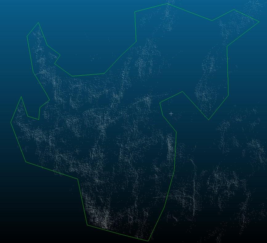
32 Methods Referring to previous Chapter 5.1 and Figure 18, two forest areas (sample plots 1 3 and sample plots 4 5) near the Department of Built Environment at Aalto University were laser scanned. These scans were used as the material for evaluating and comparing tree identification methods tested in this study. All the five sample plots were modelled. These models are shown in Figures Each of these models consists of several point clouds acquired from several scanning stations and registered to one single point cloud using Faro Scene software. To achieve a diverse, comprehensive, and yet a compact point cloud, the first three sample plots (plots 1 3) were scanned by laser scanning only, and the two last plots (plots 4 5) were scanned with a RGB-assisted method Tree positioning The reference data for tree positioning was acquired manually based on the classification of each registered point cloud into the tree trunks at the DBH. The measurement of the stems was performed by the Terrascan program, a subprogram of MicroStation. In this program, the mouse arrow was focused on the centres of the point set representing the stem cross-section. A circle was manually fitted to the point set corresponding to the stem. Consequently, the tree coordinates and DBHs were able to be accurately measured and used as reference data for the tree locations and DBHs achieved by automatic cylinder fitting performed in Matlab. Thus, the accuracy and the reliability of the tree positioning based on the cylinder fitting could be evaluated. The tree species identification was based on the manually measured tree structure parameters. The reference data of tree species utilised in the classification was based on checking the species in the sample plots. Figure 19: Sample plot 1 visualised by intensities.

33 27 Figure 20: Sample plot 2 visualised by intensities. Figure 21: Sample plot 3 visualised by intensities.

34 28 Figure 22: Sample plot 4 visualised by RGB-values. Figure 23: Sample plot 5 visualised by RGB-values. The scans of the sample plots acquired by the scanners were imported in the Faro Scene program from the scanner memory in format e57. This format consists of the XYZ-coordinates and the intensities of the point cloud points. The clouds were registered to the common coordinate system by Faro Scene. Thus, the unambiguous coordinates for the

35 29 trees were definable. The registered data sets were separately exported by Faro Scene in XYZ-coordinate format. These formats, in turn, were exported to las-format by the program CloudCompare. Only one or two scans from each sample plot were imported in CloudCompare because the capability of the program to process the whole data set is limited. Las-formats were used by TerraScan for classifying the point clouds. The extraction of the point set representing the stem cross-section was performed by clipping each tree manually to a slice at the DBH. This was performed with the CloudCompare program. Tree positioning was implemented by fitting a cylinder to the points forming the extracted slice. The tree locations and DBHs determined by the cylinder fitting were compared with the manually measured reference position and DBH data provided by the Terrascan. In following, the tree identification process is described in more detail. In the registered point clouds, the tree stems were separated from the crowns and terrain surface by the classification algorithms used by TerraScan. Thus, the point clouds representing the stem cross sections were achieved. Terrascan was utilised to import and process all scans or only a part of the scans in las-format. Usually, Terrascan is not able to process very large data sets. Therefore, only a tenth of each sample plot cloud points was chosen for the processing. The first step performed on the point cloud imported to the Terrascan was the classification of the cloud points into terrain (Figures 23 and 24). Figure 23: Initial data including all laser points.

36 30 Figure 24: Initial data classified into the terrain surface as shown by orange-coloured points. Next, the stem cross-sections at breast height were separated by Terrascan from the original point cloud. As the result, the cross-sections of the tree stems at breast height ( metres from the ground) were achieved (Figure 25). This figure representing a map in Terrascan, was needed to approximately measure the reference values for tree positions and DBHs. The point cloud represented by Figure 26 was, in turn, needed to identify each tree by pencil when visiting the sample plots. This point cloud had been bounded manually in vertical direction to the same cross-sections as shown in Figure 25. The clipping box tool from Faro Scene was used to bound the original point cloud representing the trunks from each sample plot. The clouds were vertically bounded to breast height, showing enough of same tree stems as in the map created by Terrascan (see Figures 25 and 26). The point cloud in Figure 26 was bounded from the original point cloud by Faro Scene to the stems and was printed. The tree identification numbers (ID) and tree species were signed to this print by pencil when visiting the sample plot. The trunk cross-sections were labelled as shown in the map achieved by Terrascan (Figure 26). Then, the clipping box tool in Faro Scene was utilised to vertically extend the point cloud to show the tree crowns (Figure 27). Thus, the correctness of the manually labelled trees could be checked. The reference tree location data determined by Terrascan (Figure 25) and the tree ID:s and species information signed to the prints (Figure 26) were combined and registered as shown in Tables 2 6.

37 31 Figure 25: An example of a map created by Terrascan showing stem cross-sections as green circles. Figure 26: Cross-sections of the tree stems achieved by the clipping box tool in Faro Scene.

38 32 Figure 27: Bounding of the point cloud by the clipping box tool in Faro Scene. The next step was to measure the tree positions by zooming the cursor approximately to the stem centre and registering the centre X- and Y-coordinates (Figure 28). Then, the visual circle fitting to the point set representing the trunk cross-section was performed (Figure 29). The circle was searched by iteration. In this procedure, the circle was visually placed to stem points so that the circle fits to the point set. The average DBH was calculated from two best-fitted circles. The DBHs for both circles were measured by placing a dashed line through the trunk centre (Figure 30). The reference data of the tree locations and DBHs measured from each sample plot were registered as shown in the Tables 2 6.

39 33 Figure 28: X- and Y-coordinates measured from the stem centre at the DBH. Figure 29: The circle fitting to the point set.

40 34 Figure 30: Measuring the DBH. The reference measurements from Sample Plot 1 are shown in Table 2. The table shows the IDs, positions, and DBHs of eight birches, three pines, and five spruces in Sample Plot 1. For Tree 3, the stem cross-section was so slightly visible in Terrascan that the circle fitting was unreliable, thus giving impossible results for the DBHs. Table 2: Tree locations and DBHs in Sample Plot 1.

41 35 The reference measurements from Sample Plot 2 are recorded in Table 3 showing the IDs, positions and DBHs of two birches and two spruces. Table 3: Tree locations and DBHs in Sample Plot 2. The reference measurements from Sample Plot 3 are recorded in Table 4 showing the IDs, positions and DBHs of six birches and four spruces. Table 4: Tree locations and DBHs in Sample Plot 3. The reference measurements from Sample Plot 4 are recorded in Table 5. The table shows the IDs, the positions and DBHs of eight birches, one spruce and two pines. Table 5: Tree locations and DBHs in Sample Plot 4.

42 36 The reference measurements from Sample Plot 5 are recorded in Table 6. The table shows the IDs, positions and DBHs of 10 birches, 1 spruce and 1 pine. Table 6: Tree locations and DBHs in Sample Plot 5. The accuracy and the reliability of the tree positions and the DBHs provided by the cylinder fitting (Tables 7, 9, 11, and 13) were evaluated based on the comparison to the reference values in Tables 2 6. Automatic M-estimator sample consensus (MSAC) algorithm based on the RANSAC-code (mentioned in Chapter 3.3) was used as the fitting method in Matlab R2019a. MSAC works by the same principle as RANSAC, searching enough iterations to provide a robust probability model. However, the MSAC-algorithm describes the reliability of the model based on the least squares method determined by the errors. (Mathworks 2019c, Sangappa & Ramakrishnan 2019, 72-73) The cylinder fitting was performed by Matlab to a tree stem slice, representing tree stem cross-section at breast height. The vertical thickness of the slice was approximately 10 cm and was cut from the las-file exported by CloudCompare. This slice extended approximately 5 cm upwards and downwards from the DBH (Figure 31). The breast height (1.3 m) was visually measured from the terrain by the cutting tool. Figure 31: Tree stem bounded by the cutting tool in CloudCompare.

43 37 The cylinder fitting was performed separately for each tree by a Matlab-code. The first step in the code was to read the point set of the extracted slice from the tree stem by command las-data('puu1.las', 'loadall'). Then, the algorithm accomplished the cylinder fitting by Matlab function pcfitcylinder(). This routine is based on the MSAC-algorithm fitting a cylinder to the point set by leaving the maximum distance of five millimetres between the points and the cylinder. (Mathworks 2019c) The fitting result was determined by the command pcfitcylinder (ptcloud,maxdistance,referencevector,'sampleindices',sampleindices). The routine in question also takes into account the angle of the gradient between the fitted circle and the horizontal plane of the point set. The orientation was set by the reference vector [0 0 1] in which the last element is the one-degree angle of the gradient. (Mathworks 2019c) The cylinder (Figure 32) fitted to the point set shown in Figure 31 enabled the X- and Y- coordinates of the extracted stem slice to be determined. The coordinates were defined in the scanner model coordinate system. The other output parameters provided by the cylinder fitting code were the tree DBH and the offset distances of the slice points from the fitted cylinder. Figure 32: Cylinder fitted to the point set representing the part of the tree stem at the DBH Identification of tree species The next step was to identify the tree species based on the tree structure parameters (Figure 14 and 15) and the intensities. The identifiable trees comprised of three different tree species, with three trees representing each species. Thus, the sample consisted of three birches, three spruces, and three pines. Only nine trees were sampled to the classification.

44 38 It was difficult to measure the structure parameters of all trees because most of the tree crowns occluded each other. The sampled trees with reference DBHs were chosen from Tables 2 6. It was more reliable to utilise the earlier in Terrascan measured DBHs than to measure the DBHs separately in CloudCompare. The other structure parameters (Figure 14) could be measured in CloudCompare by the cutting tool. To measure the tree parameters, the point cloud was bounded to a clearly distinguishable tree and its measurements. Each parameter was measured separately. Figure 33 shows the height of a pine measured with cutting tool. Correspondingly, the crown measurements were determined and read from the tool showing crown widths in X- and Y-directions in metres (Figure 34). Also, the other structure parameters (Figure 14) were measured with the same method. The measured parameters were used to calculate the values defined in Figure 15. All measured and calculated structure parameters were registered to the Tables Figure 33: The height of a pine bounded by the cutting tool.

45 39 Figure 34: The pine in Figure 33 with the diameters in X- and Y-directions as defined by the cutting tool. Next, the intensity data from the test tree stems and crowns were acquired. In addition to the tree structure parameters, these intensity data were used in feature vectors characterizing the tree species. First, the scans of Sample Plots 1 and 2 recorded as e57- formats were registered by Faro Scene to the same coordinate system as a single e57-file. Thus, the trees were founded easily based on the comparison of the crowns in las- and e57-files. However, part of the trees from Plot 4 was sampled because the trees were clearly distinguishable and their structure parameters were relatively reliably measurable. Although the scans acquired from this plot comprised the intensities and the RBG-values, Faro Scene assumed only the colour values as the interests. Consequently, the scanning files with e57-formats were not enabled to register as a single file directly as mentioned above. The intensity values acquired from Plot 4 were achieved from fls-files that were registered by Faro Scene into the common coordinate system and exported as an e57-file. Thus, the intensities from Plot 4 were sighted and the test trees on the plot could be located. All sample plots were surveyed in the fall, so the deciduous trees lacked leaves. The next step was to extract the intensity data from test tree stems and foliages by cutting a point set from the stems and crowns (Figures 35 and 36). Each extracted point data set were saved in txt-format. Matlab could read the trunk and foliage intensity data covered by these files.

46 40 Figure 35: Extraction of the stem intensity data using the cutting tool. Figure 36: Extraction of the crown intensity data using the cutting tool.

47 41 The tree identification was based on the k-means -algorithm utilising the tree structure parameters. The algorithm was processed by Matlab. The k-means -method is based on the clustering of observations. The clusters refer to the desired number of groups (e.g., three different tree species). The algorithm separately considers the observation parameters corresponding to the same feature of each tree. First, a desired given value was set for the average of these parameters. Next, each of these parameters was explored one by one, and was set to the cluster with the average value nearest to given value. The clustering was continued until each observation moved enough close to the average feature vectors. Figure 37 represents an example of point clustering. (Mathworks 2019d) Figure 37: Example of point clustering based on data values. (Mathworks 2019d) The cluster labelling by tree species was performed manually. The considered factors utilised in the clustering are presented as structure parameters in Figure 14, ((Crown length)/(tree height), DBH/(tree height), FLBH/(tree height), Branch angle, (Crown length)/(crown diameter), (Tree height-lls)/(tree height-hls), LS/LCS, and (Mean height for all of the grids)/(tree height), Side gap fraction for all of the grids, Leaf area index for all of the grids,) and the stem and foliage intensities. A code based on the k- means -algorithm was applied in Matlab (Appendix 1) to explore tree classification into the correct species. The classification accuracy was evaluated separately by three groups of data: structure parameters only, simultaneously structure parameters and the intensities, and the intensities only. The given values of the classes were moved in these classification cases. The aim of the initial feature vectors for k-means was to ensure the unambiguity of the tree species classification. Due to the small size of the sample plot, the different starting values for initial feature vectors changed the results.

48 Results In this chapter, the results of this study are presented. First, the results concerning tree stem locations and DBHs are shown. Then, the tree species classification are described Tree locations and DBHs This chapter represents the locations and DBHs of the test trees in Sample Plots 1 5 provided by the automatic cylinder fitting. The results achieved by automatic cylinder fitting are shown in Tables 7, 9, 11, and 13. The results in Tables 7, 9, 11, and 13 achieved by the automatic cylinder fitting method were compared with the manually measured results in Tables 2 6. The results of this comparison are shown in Tables 8, 10, 12, 14, 16, and 17. The results for different sample plots are shown below. Sample Plot 1: Table 7 shows the XY-coordinates, DBHs of trees 1 and 15, and the offset distances between the stem points and the fitted cylinder from Sample Plot 1. Table 8 shows the corresponding information with the comparison data. Table 7: Trees 1 and 15 and their data from Sample Plot 1 Table 8: Sample Plot 1 comparison data Sample Plot 2: Table 9 shows the XY-coordinates, DBHs of trees 1 4, and the offset distances between the stem points and the fitted cylinder from Sample Plot 2. Table 10 shows the corresponding information with the comparison data.

49 43 Table 9: Trees 1 4 and their data from Sample Plot 2 Table 10: Sample Plot 2 comparison data Sample plot 3: Table 11 shows the XY-coordinates, DBHs of trees 2 4, and the offset distances between the stem points and the fitted cylinder from Sample Plot 3. Table 12 shows the corresponding information with the comparison data. Table 11: Trees 2 4 and their data from Sample Plot 3 Table 12: Sample Plot 3 comparison data

50 44 Sample plot 4: Table 13 shows the XY-coordinates, DBH:s of trees 1,6,7 and 12, and the offset distances between the stem points and the fitted cylinder from sample plot 4. Table 14 shows the corresponding information with comparison data. Table 13: Trees 1,6, 7 and 12, and their data from Sample plot 4 Table 14: Sample plot 4 comparison data. Sample plot 5: Table 15 shows the XY-coordinates, DBH of tree 2, and the offset distances between the stem points and the fitted cylinder from Sample Plot 5. Table 16 shows the corresponding information with the comparison data. Table 15: Tree 2 and its data from Sample Plot 5 Table 16: Sample plot 5 comparison data.

51 45 Table 17 shows the overall error data determined from each sampled tree. Table 17: Overall error data Tree species classification Tables show the parameters utilised in tree identification. The classification parameters were branch angle and the five lowest parameters in the table LCHT, DSHT, LCDEA, LLLSLHLS, and LSLCS. Table 18 shows the structure parameters of three birches. The 10 uppermost parameters in the table were measured using CloudCompare. The five lowest parameters were determined utilising these 10 parameters. Table 18: Birch structure parameters The structure parameters of three spruces considered in Table 19 corresponded to those in the previous case.

52 46 Table 19: Spruce structure parameters The structure parameters of three pines were considered in Table 20 corresponded to those in the previous case. Table 20: Pine structure parameters In addition to the tree structure parameters, the median intensities determined separately from each tree trunk and foliage intensities were used in tree species classification (Tables 21 23).

53 47 Table 21: Birch intensities Table 22: Spruce intensities Table 23: Pine intensities The best classification result provided by Matlab-code based on k-means -algorithm was achieved by the procedure of simultaneously using the structure parameters (five bottom values in Tables 18 20) and the intensities (Tables 21 23). The same classification result was provided using the structure parameters only. According to these results, the three birches and three spruces were correctly classified. However, two of the three reference pines were incorrectly classified into birches. Thus, the following error matrix for both cases mentioned above was formed. Birch Spruce Pine Birch Spruce Pine Classification by only median intensity values of tree stems and foliages (see Tables 21-23) correctly identified all spruces. However, only one of three birches was correctly classified. Two of the birches were misidentified as spruces. In addition, although two of the three pines were correctly classified and one pine was misidentified as a spruce. Thus, the following error matrix was formed. Birch Spruce Pine Birch Spruce Pine 0 0 2

54 Analysis The results provided by the cylinder fitting and manual measurements were analysed using different error parameters. The evaluation was based on the overall errors of the X- and Y-coordinates, DBHs, and positions of the trees. Moreover, the mean errors, standard errors, and standard deviations of the same parameters were determined. The standard errors were calculated to show also the largest deviations. The standard deviations, in turn, indicate the average deviation from the expected value of the error. These factors were calculated separately for each sample plot and finally an overall value was calculated for all the sampled trees. Tables 8, 10, 12, 14, and 16 show the errors of X- and Y-coordinates, DBHs, and overall location determined for the trees sampled separately from Sample Plots 1 5. The error evaluation was performed separately for each sample plot also based on the mean errors, standard errors, and standard deviation of the corresponding parameters (Tables 8, 10, 12, 14, and 16). Finally, the overall biases between the cylinder fitting and manually measured results were evaluated. Table 17 shows the overall mean errors, standard errors, and standard deviations of X- and Y-coordinates, DBHs, and location determined from all sampled trees. All parameters mentioned above refer to the maximum deviation in centimetres. Thus, the results appear to be credible. The only considerable biases appear in the X-coordinate and overall location of tree 6 from Sample Plot 4 exceeding one decimetre. Furthermore, the Y-coordinate and the position of tree 2 from Sample Plot 5 have a relatively large bias. These deviations may be explained by the relatively large tree angle of the gradient. Moreover, the ground elevation variates considerably. The point cloud was acquired from higher positions. Thus, the terrain surface and the tree stem were not covered so well by the registered point cloud. Consequently, discerning the boundary between the ground surface and the tree stem in CloudCompare may be challenging. Possibly, these issues also hampered the bounding and extraction of the sample slice from the DBH. Furthermore, due to the tree angle of gradient, a small difference in DBH already significantly affected the tree location. According to the parameters shown in Table 17, the overall positioning accuracy seems to be quite well succeeded. Even the largest overall deviations shown by the root-meansquare error and the average deviations from the expected value shown by standard deviations seem to be fairly low. However, the precision of the cylinder fitting and the results provided might be considerably higher if all of the scans acquired from each sample plot were utilised. Unfortunately, the accuracy evaluation only included one or two scans due to the limited processing capacity of the computer. Each tree stem could not be covered with this number of scans. Consequently, the circle fitting performed for the stems may be relatively inaccurate. Furthermore, each tree with reference coordinates and DBHs measured in Terrascan did not appear in CloudCompare because some of the stems merged with the foliage. Thus,

55 49 the cylinder fitting was not performable for as many trees expected. This issue made for a relatively reduced evaluation of the cylinder fitting. Figures describe the geometry of different tree species utilised for tree classification. Only birches and pines are shown in the figures because they could not be classified by programming-based computation reliably. The computation mixed a part of the trees with each other. Instead of that, the classification of spruces proved to be reliable and occurred correctly. Spruces could be separated from other tree species. A more exact explanation for the figures are described after the images. Figure 38: Birch1 Figure 39: Birch 2 Figure 40: Birch 3 Figure 41: Pine 1 Figure 42: Pine 2 Figure 43: Pine 3